Download

1 / 43
440 likes | 749 Views
ANOVA Analysis of Variance. The Plan for Today. Basics of parametric statistics ANOVA – Analysis of Variance T-Test and ANOVA in SPSS Lunch T-test in SPSS ANOVA in SPSS. Parametric statistics. What kind of data can we analyse using parametric statistics ?.

E N D
The Plan for Today • Basics of parametric statistics • ANOVA – Analysis of Variance • T-Test and ANOVA in SPSS • Lunch • T-test in SPSS • ANOVA in SPSS
What kind of data canwe analyse usingparametricstatistics? • The arithmetic mean can only be derived from interval or ratio measurements. • Interval data – equal intervals on a scale; intervals between different points on a scale represent the difference between all points on the scale. • Ratio Data – has the same property as interval data, however the ratios must make mutually sense. Example 40 degrees is not twice as hot as 20 degrees; reason the celsius scale does not have an absolute zero.
Whencanweuseparametricstatistics? • Assumption 1: Homogeneity of variance – means should be equally accurate. • Assumption 2: In repeated measure designs: Sphericity assumption. • Assumption 3: Normal Distribution
Parametric statistics • Assumption 1:Homogeneity of variance • The spread of scores in each sample should be roughly similar • Tested using Levene´s test • Assumption 2:The sphericityassumption • Tested using Mauchly´s test • Basically the same thing:homogeneity of variance
When is a distribution far enough from normal to become a problem? • Assumption 3: Normal Distribution. • In SPSS this can be checked by using: • Kolmogorov-Smirnov test • Shapiro-Wilkes test • These compare a sample set of scores to a normally distributed set of scores with the same mean and standard deviation. • If (p> 0.05) The distribution is not significantly different from a normal distribution • If (p< 0.05) The distribution is significantly different from a normal distribution
Analysis of Variance • Difference between t-test and ANOVA: • t-test is used to analyze the difference between TWO levels of an independent variable. • ANOVA is used to analyze the difference between MULTIPLE levels of an independent variable.
Analysis of Variance • Independent variable = apple • Dependent variables could be: sweetness, decay time etc. t-test ANOVA …or more
Analysis of Variance • The ANOVA tests for an overall effect, not the specific differences between groups. • To find the specific differences use either planned comparisons or post hoc test. • Planned comparisons are used when a preceding assumptions about the results exists. • Post Hoc analysis is done subsequent to data collection and inspection.
Analysis of Variance • A Post Hoc Analysis is somewhat the same as doing a lot of t-tests with a low significance cut-of point, the Type I error is controlled at 5%. • Type I error: Fisher’s criterion states that there is a o.o5 probability that any significance is due to diversity in samples rather than the experimental manipulation – the α-level. • Using a Bonferroni correction adjusts the α-level according to number of tests done (2 test = o.5/2 = 0.025. 5 test= 0.5/5= 0.01). Basically the more tests you do the lower the cut of point.
The logic of an ANOVA • Variation in a set of scores comes from two sources: • Random variation from the subjects themselves (due to individual variations in motivation, aptitude, etc.) • Systematic variation produced by the experimental manipulation.
F-ratio • ANOVA compares the amount of systematic variation to the amount of random variation, to produce an F-ratio: systematic variation F = random variation (‘error’)
F-ratio • Large value of F: a lot of the overall variation in scores is due to the experimental manipulation, rather than to random variation between subjects. • Small value of F: the variation in scores produced by the experimental manipulation is small, compared to random variation between subjects.
Calculations I • In practice, ANOVA is based on the variance of the scores. The variance is the standard deviation squared: variance
Calculations II • We want to take into account the number of subjects and number of groups. Therefore, we use only the top line of the variance formula (the "Sum of Squares", or "SS"): • We divide this by the appropriate "degrees of freedom" (usually the number of groups or subjects minus 1). sum of squares
Three types of SS (sum of squares) • Between groups SSM: a measure of the amount of variation between the groups. (This is due to our experimental manipulation).
Three types of SS (sum of squares) • Within GroupsR: a measure of the amount of variation within the groups. (This cannot be due to our experimental manipulation, because we did the same thing to everyone within each group).
Three types of SS (sum of squares) • Total sum of squares:a measure of the total amount of variation amongst all the scores. (Total SS) = (Between-groups SS) + (Within-groups SS)
Significance of F-Ratio • The bigger the F-ratio, the less likely it is to have arisen merely by chance. • Use the between-groups and within-groups d.f. to find the critical value of F. • Your F is significant if it is equal to or larger than the critical value in the table.
Here, look up the critical F-value for 3 and 16 d.f. Columns correspond to between-groups d.f.; rows correspond to within-groups d.f. Here, go along 3 and down 16: critical F is at the intersection. Our obtained F, 25.13, is bigger than 3.24; it is therefore significant at p<.05. (Actually it’s bigger than 9.01, the critical value for a p of 0.001).
Overview • One –Way ANOVA • Independent • Repeated Measures • Two-way ANOVA • Independent • Mixed • Repeated Measures • N-way ANOVA
One-Way Independent ANOVA • One-Way: ONE INDEPENDENT VARIABLE • Independent: 1 participant = 1 piece of data. Independent variable: Yoga Pose,3 levels Dependent variables: Heart rate, oxygen saturation
One-Way Dependent ANOVA • One-Way: ONE INDEPENDENT VARIABLE • Dependent : 1 participant = Multiple pieces of data. Independent variable:Cake,3 levels Dependent variables: Blood sugar, pH-balance
Two-Way Independent ANOVA • Two-Way : TWO INDEPENDENT VARIABLES • Independent : 1 participant = 1 piece of data. Independent variables: Age, Music Style >40 <40 Indie-Rock Classic Pop
Two-Way Mixed ANOVA • Two-Way : TWO INDEPENDENT VARIABLES • Mixed: • Variable 1: Independent (Controller) • Variable 2: Repeated measures (Space Ship)
Two-Way Dependent ANOVA • Two-Way: TWO INDEPENDENT VARIABLES • Dependent : 1 participant = Multiple pieces of data. Independent variables: Exercise, Temperature 30 ° 20 ° 25 °
SPPS SPSS
Click ‘Options…’ Then Click Boxes: Descriptive; Homogeneity of variance test; Means plot
Things to remember • One-way independent-measures ANOVA enables comparisons between 3 or more groups that represent different levels of one independent variable. • A parametric test, so the data must be interval or ratio scores; be normally distributed; and show homogeneity of variance. • ANOVA avoids increasing the risk of a Type 1 error.