Download
1 / 72
720 likes | 739 Views
Explore the impact of large-scale motions on galaxy evolution focusing on Virgo Infall, nonlinear models, Hubble constants, density parameters, and the Great Attractor. Learn about galaxy biasing, velocity perturbations, and the dynamics of galaxy evolution across various scales.

E N D
AY202a Galaxies & DynamicsLecture 21:Large Scale MotionsGalaxy Evolution
Large Scale Motions Rubin 1952 Distortions deVaucouleurs 1956 Local Supergalaxy Supercluster Rubin, Ford, Thonnard, Roberts 1976 + answering papers Peebles – Silk – Gunn early ’70’s Mass and Light CMB dipole 1976-79 Wilkinson++, Melchiori++ (balloons) Virgo Infall Schechter ’80, TD ’80, DH ’82, AHMST ’82 Great Attractor --- 1985 Seven Samurai (BFDDL-BTW) Kaiser 1985 Caustics IRAS Surveys 1985 Davis, Strauss, Fisher, H, ++ ORS 1992 Santiago et al.
COBE Dipole ‘97 3.358 mK towards l=264.31 & b= 48.05
Flows and Dipoles (Silk; Peebles; Gunn) Gravity g ~ M/R2 Light f ~ L/R2 So, if <M/L> ~ constant Gravity Vector = Flux Vector
The Infall S-Curve First Target Virgo Infall
Virgo Infall Schechter 1980 Faber Jackson on 32 E’s Virgo Infall 190+/-130 km/s Linear Infall Model for any given galaxy V0bs = VVirgo x - w(cos θ –x) [1 – (x2 -2x cosθ +1) –γ/2] x = distance to galaxy in Virgo Units Virgo has a density contrast that falls as d-γ w is the LG infall velocity to Virgo d is the galaxy’s distance from Virgo θ is the angular separation between Virgo & the galaxy
Nonlinear Model (Schechter ’80; Silk ’74, ’77) Treat each shell around Virgo as its own Universe with its own average interior density and Hubble Constant and own present density parameter . Define the Friedmann arc parameter η cosh-1(2/ -1) for < 1 cos-1(2/ -1) for > 1 & define also the functions h (η) = ρ (η) = for > 1 η = { sin η (η – sin η) (1 cos η)2 (η – sin η)2 (1 – cos η)3
and similar sinh functions for < 1, then if ηu is the present universal value of the arc and ηg is the value for the shell or a particular galaxy g then the ratios of the local Hubble constant and the average interior density to the universal H and average density are given by h(ηg) / h(ηu) and ρ(ηg) / ρ(ηu) and VObs = VVirgo ( ) and the subscript l refers to the Local Group hu x – (hu –hl)cosθ – (x – cosθ) (hu – hg) hg
Once ρl/ρu and γ are specified, only ρu needs to be set to determine all the h’s to also be specified. Determining w determines ρu and thus w = (hu/hl -1) VVirgo VVirgo is the Virgo velocity corrected for infall and any remaining peculiar LG velocity
Accurate Motions AMHSSB ‘80 Ten Clusters
V0bs = VHubble + VPeculiar + VGrav we can neglect the gravitational redshifts of galaxies, then VPeculiar = VPattern + VRandom and VP/VH = -1/3 0.6 (Δ - 0.19Δ2 + …..) where Δ = δρ/ρ, the overdensity inside 0.6 ~ 3 ( ) ( )-1 ( 1 + ….) VP δρ VH ρ
Velocity Perturbations from TF fit to a Virgo Infall Model AHMST 1982 z residuals, no infall V infall ~ 250 km/s w.r.t. Hubble Flow
The Great Attractor Seven Samurai – Lynden-Bell, Faber, Davies, Dressler, Burstein, Terlevich & Wegner Faber-Jackson • Dn-σ on 400 E’s found 570 +/- 60 km/s towards Centaurus
Problems ---- (1) Virgo ≠ CMB (2) Hydra-Cen ≠ CMB (3) GA + Virgo ≠ CMB amplitude (4) Honkin’ Pisces-Perseus on the other side (5) Where is Convergence? (6) Biasing
Galaxy Bias If galaxies don’t trace the mass and the galaxy overdensity is not the mass overdensity, one can use the simple linear biasing model So usually the results of flow field analyses are quoted in terms of f() 0.6 / b δρ 1 δn ρ b n =
What is the ideal All-Sky Survey? Go to the near IR! ---- Beat extinction, the bane of optical surveys --- Select for the stars that trace the baryonic mass (not star formation)
Magenta V < 1000 km/s • Blue 1000 < V < 2000 km/s • Green 2000 < V < 3000 km/s
Red3000 < v < 4000 Blue 4000< v < 5000 Green 5000 < v < 6000
Red 6000 < v < 7000 Blue 7000 < v < 8000 Green 8000 < v < 9000
Great Wall LSC We are here Pisces-Perseus KS < 11.25
2MRS Dipole blue tri = FW - M81, Maffei’s & friends(Erdogdu et al 2006) red tri = FW - only LG
Density vs Flow Fields Don’t do this! Much Better! CMB versus LG Reference Frames
Hectospec Positioner on MMT 300 Fibers covering a 1 degree field of view D. Fabricant
Large Synoptic Survey Telescope 8.4-m 7 degree FOV
Galaxy Evolution Galaxies Evolve! A. Population Evolution (Stars) B. Gaseous Evolution A + B = Chemical Evolution C. Dynamical Evolution There is strong evidence for all three
A – we see galaxies with both young and old stellar populations and with current star formation\ B – we see infall (e.g. MW high velocity clouds) and outflow (M33) and cooling flows A+B we see correlations between stellar age and stellar [Fe/H] in the MW. Abundance gradients in other spirals C – we see mergers, cannibalism, interactions, dynamical friction Basically L, D, U-B, B-V, … L(r,θ), F(λ), Φ(L) all change with time.
Population Evolution Tinsley ‘68, SSB ’73, JPH ’77 and the death of the Hubble/Sandage cosmology program … The Flux from a galaxy at time t and in band i is FG(i,t) = [ Ψ(k,j) ∫ FK(i,t’) dt’ ] where FK(i,t’) is the flux of star of type k in bandpass i at age t’ and ∫ F is the integrated flux in the jth timestep n-1 (n-j)Δt j k (n-j-1)Δt
This is piecewise, time-weighted summation in an Age-Flux table for stars Ψ(k,j) is the birth rate function of stars of type k in the jth time step Ψ(k,j) Ψ(m,t) = m–α e–βt The Initial Mass Function (IMF) is often parameterized as m–α with α = 2.35 as the Salpeter slope The Star Formation Rate (SFR) is often parameterized as an exponential in time R(t) = A e–βt or as R(t) = m0/τ e–(t/τ)τ = 1 Bruzual “C” Model = 1 - e– (1 Gyr / τ)