Download
1 / 9
90 likes | 251 Views
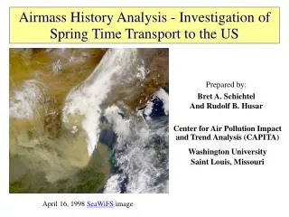
Airmass History Analysis - Investigation of Spring Time Transport to the US. Prepared by: Bret A. Schichtel And Rudolf B. Husar. Center for Air Pollution Impact and Trend Analysis (CAPITA) Washington University Saint Louis, Missouri. April 16, 1998 SeaWiFS image. Introduction.

E N D
Airmass History Analysis - Investigation of Spring Time Transport to the US Prepared by: Bret A. SchichtelAnd Rudolf B. Husar Center for Air Pollution Impact and Trend Analysis (CAPITA) Washington University Saint Louis, Missouri April 16, 1998 SeaWiFS image
Introduction • On April 15th, 1998 an unusually intense dust storm began in the western Chinese Province of Xinjiang. By April 20, the dust front covered a 1000 mile stretch on the east coast of China and within five days it moved across the Pacific impacting the West Coast. • This event was closely monitored by the air quality community using satellite, aircraft and surface based measurements. • A number of organizations have taken advantage of this unique “natural tracer experiment“ to test and validate global transport models, including the Naval Research Laboratory, Euro-Mediterranean Centre on Insular Coastal Dynamics and NOAA’s Climate Monitoring & Diagnostics Laboratory. • This analysis adds to the body of the Chinese dust simulations by simulating the transport of the Chinese dust cloud from April 19 – April 30 using the CAPITA Monte Carlo Model driven by the FNL global meteorological data. The simulation is evaluated against TOMS aerosol index and surface PM10 and PM2.5 measurements.
CAPITA Monte Carlo Model A diagnostic tool that uses the Monte Carlo approach to simulate and investigate the roles of air pollutant emissions, transport and kinetics on air quality. • An airmass is represented by a number of quanta or particles • The individual particles are subjected to transport, transformation and removal processes, with mass conservation maintained at the particle level. • Dispersion, forward or backward in time, is represented by the advection and spread of the particles. • Dispersion proceeds independently from the nature and chemistry of the pollutants
CAPITA Monte Carlo Model - Transport Advection:Particles are moved in 3-D space using the input meteorological data’s mean wind field. Horizontal Dispersion:Eddy diffusion coefficients, which vary depending on time of day, randomly displace the particles horizontally. Vertical Dispersion:Intense vertical mixing within the mixing layer is simulated by uniformly distributing particle from the ground to the mixing height. No vertical dispersion is applied to particles above mixing layer.
CAPITA Monte Carlo Model - Kinetics Chemistry:Pseudo first order transformation rates, function of meteorological variables, such as solar radiation, temperature, water vapor content Deposition dry and wet:Pseudo first order rates equationsDry deposition function of hour of solar radiation, Mixing Hgt Wet deposition function of precipitation rate Note: in this application no kinetics were applied to the particles
FNL Meteorological Data Archive The FNL data is a product of the Global Data Assimilation System (GDAS), which uses the Global spectral Medium Range Forecast model (MRF) to assimilate multiple sources of measured data and forecast meteorology. • 129 x 129 Polar Stereographic Grid with ~ 190 km resolution. • 12 vertical layers on constant pressure surfaces from 1000 to 50 mbar • 6 hour time increment • Upper Air Data: 3-D winds, Temp, RH • Surface Data includes: pressure, 10 meter winds, 2 meter Temp & RH, Momentum and heat flux • Data is available from 1/97 to present.
FNL Meteorological Data Processing • The Monte Carlo model requires the input meteorological data to have a terrain following vertical coordinate system and an estimate of the mixing height. Therefore, the data were reprocessed: • The vertical coordinate system was converted from constant pressure surfaces to 18 constant height surfaces above the ground from 10 to 11000 meters. The 10 meter winds and 2 meter temperature and RH surface variables were incorporated into the upper air variables. • The vertical velocity was converted from mbar/sec to meter/sec. • An estimate of the mixing layer height was computed from a modified bulk Richardson number that accounts for mixing due to convective and mechanical processes. The mixing height was limited to 4 km.
Receptor Site Latitude Longitude Seattle, WA 47.6 122.33 San Francisco, CA 37.78 122.42 San Diego, CA 32.72 117.15 Minneapolis, MN 44.98 93.27 St. Louis, MO 38.62 90.2 San Antonio, TX 29.42 98.5 Boston, MA 42.37 71.07 Norfolk, VA 36.85 76.28 Miami, FL 25.78 80.18 US Airmass Histories • Fifteen day airmass histories for 9 receptor sites were calculated every two hours from February – April 1999. • Each airmass history is composed of 15 trajectories which are tracked at two hour time increments back in time. • The trajectory starting heights are within the mixing layer. • The following variables are saved out along each trajectory: Temperature, Relative Humidity, Cloud coverage, Precipitation rate, and Mixing height. • Horizontal and vertical mixing are used in the airmass history calculations.
Conclusions • A Monte Carlo simulation was used to simulate the horizontal and vertical transport of the April 19 Chinese Dust Cloud. The simulation showed: • The dust cloud split into two airmass with the northern airmass entrained in a low pressure system that was rapidly transported to the West Coast and the southern airmass entrained in a high pressure system that stalled in the middle of the Pacific. • The dust cloud was formed at the surface and by April 20, its front was elevated to 4-10 km. The northern part of the dust cloud remained elevated until it reached the west coast where it descended impacting the surface between April 27-28. • The CAPITA Monte Carlo Model driven by the FNL winds was able to reproduce the dust cloud pattern as it was transport from Asia to the US as identified by the TOMS data. • The simulation correctly identified the time the dust cloud descended to the surface at the west coast.