Intro to ANOVA
Intro to ANOVA. What Is ANOVA?. Analysis of Variance. This is a hypothesis-testing procedure that is used to evaluate mean differences between two of more treatments (or populations). What is the difference between this and t tests? ANOVA allows us to look at more than two groups at once.

Intro to ANOVA
E N D
Presentation Transcript
What Is ANOVA? • Analysis of Variance. • This is a hypothesis-testing procedure that is used to evaluate mean differences between two of more treatments (or populations). • What is the difference between this and t tests? • ANOVA allows us to look at more than two groups at once.
Some Terminology • In analysis of variance, the variable (independent or quasi-independent) that designates the groups being compared is called a factor. • The individual conditions or values that make up a factor are called the levels of the factor.
Formulae • SSw = (Xij – X.j)2 • SSbet = nj (X.j – X..)2 • SStot = (Xij – X..)2 • MSw = SSw/dfw • MSb = SSb/dfb • F = MSb/MSw
Looking At Error • The F statistic is calculated by comparing the error between groups (theoretically due to the treatment effect) to the error within groups (theoretically due to chance, or error). We look to see if differences due to our treatment effect is proportionally greater than differences due to chance alone.
Effect Size • For ANOVA we use eta squared • 2 • Calculated • 2 = SSbetween/SStotal
Post Hoc Tests • These are additional hypothesis tests that are done after an ANOVA to determine exactly which mean differences are significant and which are not. • If you reject the null, and there are three or more treatments, you may wish to explore which groups contain the mean differences.
Accumulation of Type I Error • Experimentwise alpha: This is the overall probability of a Type I error that can accumulate over a series of separate hypothesis tests. Typically, the experiment-wise alpha is substantially greater than the value of alpha used for any one of the individual tests.
Planned Comparisons • Planned comparisons refer to specific mean differences that are relevant to specific hypotheses the researcher had in mind before the study was conducted. • For planned comparisons, we generally don’t worry about accumulation of Type I error. • What we will do is use a smaller alpha level to test these hypotheses, often dividing alpha by the number of planned comparisons.
Unplanned Comparisons • Unplanned comparisons involve sifting through the data to find significant results. When doing this you have to worry about accumulation of Type I error in your results. Two commonly used procedures to protect against this accumulation are Tukey’s HSD and the Scheffe test.
Tukey’s HSD • Tukey’s Honestly Significant Difference (HSD) is used to compare two treatment conditions. If the mean difference between those treatment conditions exceeds Tukey’s HSD, you conclude that there is a significant difference between the treatments • HSD = q√ MSw/n • Where the value of q is found in Table B.5 (p. 708) • Tukey’s requires that n be the same for all treatments.
The Scheffe Test • Scheffe is very conservative, therefore if you use Scheffe and find a significant difference, you can feel safe you have found a true difference. • For Scheffe’s test, you calculate a serperate between groups MSb for the two groups you are looking at, and then compare this new MSb to the experimentwise MSw.
F as Compared to T • For a two sample test, an ANOVA or a t-test can be used. For these situations you would get F = t2
Assumptions • The observations within each sample must be independent • The populations must be normal • The populations must has equal variances (homogeneity of variance) • This is important to test, and we due so by Hartley’s F-max test for homogeneity of variance (table on 704) • Compute the sample variance for each sample • Divide the largest by the smallest • K is the number of samples • n is the sample size for each sample (assuming equal n’s)


