Modeling Turbulent Flows
560 likes | 1.01k Views
Gain insights into turbulent flows, modeling techniques, and efficient FLUENT training. Explore turbulence, energy cascade, DNS, LES, RANS models, and turbulence closures. Discover various turbulence models available in FLUENT for industrial applications.

Modeling Turbulent Flows
E N D
Presentation Transcript
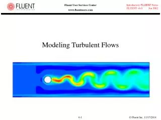
Modeling Turbulent Flows Introductory FLUENT Training
What is Turbulence? • Unsteady, irregular (aperiodic) motion in which transported quantities (mass, momentum, scalar species) fluctuate in time and space • Identifiable swirling patterns characterize turbulent eddies. • Enhanced mixing (matter, momentum, energy, etc.) results • Fluid properties and velocity exhibit random variations • Statistical averaging results in accountable, turbulence related transport mechanisms. • This characteristic allows for turbulence modeling. • Contains a wide range of turbulent eddy sizes (scales spectrum). • The size/velocity of large eddies is on the order of mean flow. • Large eddies derive energy from the mean flow • Energy is transferred from larger eddies to smaller eddies • In the smallest eddies, turbulent energy is converted to internal energy by viscous dissipation.
Is the Flow Turbulent? External Flows where along a surface around an obstacle Other factors such as free-stream turbulence, surface conditions, and disturbances may cause transition to turbulence at lower Reynolds numbers Internal Flows Natural Convection where is the Rayleigh number is the Prandtl number
Small structures Large structures Turbulent Flow Structures Energy Cascade Richardson (1922)
Overview of Computational Approaches • Reynolds-Averaged Navier-Stokes (RANS) models • Solve ensemble-averaged (or time-averaged) Navier-Stokes equations • All turbulent length scales are modeled in RANS. • The most widely used approach for calculating industrial flows. • Large Eddy Simulation (LES) • Solves the spatially averaged N-S equations. Large eddies are directly resolved, but eddies smaller than the mesh are modeled. • Less expensive than DNS, but the amount of computational resources and efforts are still too large for most practical applications. • Direct Numerical Simulation (DNS) • Theoretically, all turbulent flows can be simulated by numerically solving the full Navier-Stokes equations. • Resolves the whole spectrum of scales. No modeling is required. • But the cost is too prohibitive! Not practical for industrial flows - DNS is not available in Fluent. • There is not yet a single, practical turbulence model that can reliably predict all turbulent flows with sufficient accuracy.
Increase in Computational Cost Per Iteration Turbulence Models Available in FLUENT One-Equation Models Spalart-Allmaras Two-Equation Models Standard k–ε RNG k–ε Realizable k–ε Standard k–ω SST k–ω Reynolds Stress Model Detached Eddy Simulation Large Eddy Simulation RANS based models
RANS Modeling – Time Averaging • Ensemble (time) averaging may be used to extract the mean flow properties from the instantaneous ones: • The Reynolds-averaged momentum equations are as follows • The Reynolds stresses are additional unknowns introduced by the averaging procedure, hence they must be modeled (related to the averaged flow quantities) in order to close the system of governing equations. Example: Fully-Developed Turbulent Pipe Flow Velocity Profile Instantaneous component Time-average component Fluctuating component (Reynolds stress tensor)
The Closure Problem • The RANS models can be closed in one of the following ways (1) Eddy Viscosity Models (via the Boussinesq hypothesis) • Boussinesq hypothesis – Reynolds stresses are modeled using an eddy (or turbulent) viscosity, μT. The hypothesis is reasonable for simple turbulent shear flows: boundary layers, round jets, mixing layers, channel flows, etc. (2) Reynolds-Stress Models (via transport equations for Reynolds stresses) • Modeling is still required for many terms in the transport equations. • RSM is more advantageous in complex 3D turbulent flows with large streamline curvature and swirl, but the model is more complex, computationally intensive, more difficult to converge than eddy viscosity models.
Calculating Turbulent Viscosity • Based on dimensional analysis, μT can be determined from a turbulence time scale (or velocity scale) and a length scale. • Turbulent kinetic energy [L2/T2] • Turbulence dissipation rate [L2/T3] • Specific dissipation rate [1/T] • Each turbulence model calculates μT differently. • Spalart-Allmaras: • Solves a transport equation for a modified turbulent viscosity. • Standard k–ε, RNG k–ε, Realizable k–ε • Solves transport equations for k and ε. • Standard k–ω, SST k–ω • Solves transport equations for k and ω.
The Spalart-Allmaras Model • Spalart-Allmaras is a low-cost RANS model solving a transport equation for a modified eddy viscosity. • When in modified form, the eddy viscosity is easy to resolve near the wall. • Mainly intended for aerodynamic/turbomachinery applications with mild separation, such as supersonic/transonic flows over airfoils, boundary-layer flows, etc. • Embodies a relatively new class of one-equation models where it is not necessary to calculate a length scale related to the local shear layer thickness. • Designed specifically for aerospace applications involving wall-bounded flows. • Has been shown to give good results for boundary layers subjected to adverse pressure gradients. • Gaining popularity for turbomachinery applications. • This model is still relatively new. • No claim is made regarding its applicability to all types of complex engineering flows. • Cannot be relied upon to predict the decay of homogeneous, isotropic turbulence.
The k–ε Turbulence Models • Standard k–ε (SKE) model • The most widely-used engineering turbulence model for industrial applications • Robust and reasonably accurate • Contains submodels for compressibility, buoyancy, combustion, etc. • Limitations • The ε equation contains a term which cannot be calculated at the wall. Therefore, wall functions must be used. • Generally performs poorly for flows with strong separation, large streamline curvature, and large pressure gradient. • Renormalization group (RNG) k–ε model • Constants in the k–ε equations are derived using renormalization group theory. • Contains the following submodels • Differential viscosity model to account for low Re effects • Analytically derived algebraic formula for turbulent Prandtl / Schmidt number • Swirl modification • Performs better than SKE for more complex shear flows, and flows with high strain rates, swirl, and separation.
The k–ε Turbulence Models • Realizable k–ε (RKE) model • The term realizable means that the model satisfies certain mathematical constraints on the Reynolds stresses, consistent with the physics of turbulent flows. • Positivity of normal stresses: • Schwarz’ inequality for Reynolds shear stresses: • Neither the standard k–ε model nor the RNG k–ε model are realizable. • Benefits: • More accurately predicts the spreading rate of both planar and round jets. • Also likely to provide superior performance for flows involving rotation, boundary layers under strong adverse pressure gradients, separation, and recirculation.
The k–ω Turbulence Models • The k–ω family of turbulence models have gained popularity mainly because: • The model equations do not contain terms which are undefined at the wall, i.e. they can be integrated to the wall without using wall functions. • They are accurate and robust for a wide range of boundary layer flows with pressure gradient. • FLUENT offers two varieties of k–ω models. • Standard k–ω (SKW) model • Most widely adopted in the aerospace and turbo-machinery communities. • Several sub-models/options of k–ω: compressibility effects, transitional flows and shear-flow corrections. • Shear Stress Transport k–ω (SSTKW) model (Menter, 1994) • The SST k–ω model uses a blending function to gradually transition from the standard k–ω model near the wall to a high Reynolds number version of the k–ε model in the outer portion of the boundary layer. • Contains a modified turbulent viscosity formulation to account for the transport effects of the principal turbulent shear stress.
Large Eddy Simulationn • Large Eddy Simulation (LES) • LES has been most successful for high-end applications where the RANS models fail to meet the needs. For example: • Combustion • Mixing • External Aerodynamics (flows around bluff bodies) • Implementations in FLUENT: • Subgrid scale (SGS) turbulent models: • Smagorinsky-Lilly model • Wall-Adapting Local Eddy-Viscosity (WALE) • Dynamic Smagorinsky-Lilly model • Dynamic Kinetic Energy Transport • Detached eddy simulation (DES) model • LES is applicable to all combustion models in FLUENT • Basic statistical tools are available: Time averaged and RMS values of solution variables, built-in fast Fourier transform (FFT). • Before running LES, consult guidelines in the “Best Practices For LES” (containing advice for meshing, subgrid model, numerics, BCs, and more)
Law of the Wall and Near-Wall Treatments • Dimensionless velocity data from a wide variety of turbulent duct and boundary-layer flows are shown here: Wall shear stress where y is the normal distance from the wall • For equilibrium turbulent boundary layers, wall-adjacent cells in the log-law region have known velocity and wall shear stress data
outer layer inner layer Wall Boundary Conditions • The k–ε family and RSM models are not valid in the near-wall region, whereas Spalart-Allmaras and k–ω models are valid all the way to the wall (provided the mesh is sufficiently fine). To work around this, we can take one of two approaches. • Wall Function Approach • Standard wall function method is to take advantage of the fact that (for equilibrium turbulent boundary layers), a log-law correlation can supply the required wall boundary conditions (as illustrated in the previous slide). • Non-equilibrium wall function method attempts to improve the results for flows with higher pressure gradients, separations, reattachment and stagnation. • Similar laws are also constructed for the energy and species equations. • Benefit: Wall functions allow the use of a relatively coarse mesh in the near-wall region. • Enhanced Wall Treatment Option • Combines a blended law-of-the wall and a two-layer zonal model. • Suitable for low-Re flows or flows with complex near-wall phenomena • Turbulence models are modified for the inner layer. • Generally requires a fine near-wall mesh capable of resolving the viscous sublayer (at least 10 cells within the “inner layer”)
Placement of The First Grid Point • For standard or non-equilibrium wall functions, each wall-adjacent cell centroid should be located within the log-law layer • For enhanced wall treatment (EWT), each wall-adjacent cell centroid should be located within the viscous sublayer • EWT can automatically accommodate cells placed in the log-law layer • How to estimate the size of wall-adjacent cells before creating the grid: • The skin friction coefficient can be estimated from empirical correlations: • Use postprocessing tools (XY plot or contour plot) to to double check the near-wall grid placement after the flow pattern has been established. Flat plate: Duct:
Near-Wall Modeling: Recommended Strategy • Use standard or non-equilibrium wall functions for most high Reynolds number applications (Re > 106) for which you cannot afford to resolve the viscous sublayer. • There is little gain from resolving the viscous sublayer. The choice of core turbulence model is more important. • Use non-equilibrium wall functions for mildly separating, reattaching, or impinging flows. • You may consider using enhanced wall treatment if: • The characteristic Reynolds number is low or if near wall characteristics need to be resolved. • The physics and near-wall mesh of the case is such that y+ is likely to vary significantly over a wide portion of the wall region. • Try to make the mesh either coarse or fine enough to avoid placing the wall-adjacent cells in the buffer layer (5 < y+ < 30).
Inlet and Outlet Boundary Conditions • When turbulent flow enters a domain at inlets or outlets (backflow), boundary conditions for k, ε, ωand/or must be specified, depending on which turbulence model has been selected • Four methods for directly or indirectly specifying turbulence parameters: • Explicitly input k, ε, ω, or • This is the only method that allows for profile definition. • See user’s guide for the correct scaling relationships among them. • Turbulence intensity and length scale • Length scale is related to size of large eddies that contain most of energy. • For boundary layer flows: l 0.4 δ99 • For flows downstream of grid: l opening size • Turbulence intensity and hydraulic diameter • Ideally suited for internal (duct and pipe) flows • Turbulence intensity and turbulent viscosity ratio • For external flows: 1 <mt/m< 10 • Turbulence intensity depends on upstream conditions: • Stochastic inlet boundary conditions for LES and RANS can be generated by using spectral synthesizer or vortex method
GUI for Turbulence Models Define Models Viscous… Inviscid, Laminar, or Turbulent Define Boundary Conditions… Turbulence Model Options Near Wall Treatments Additional Options
Reattachment point Recirculation zone Example #1 – Turbulent Flow Past a Blunt Flat Plate • Turbulent flow past a blunt flat plate was simulated using four different turbulence models. • 8,700 cell quad mesh, graded near leading edge and reattachment location. • Non-equilibrium boundary layer treatment N. Djilali and I. S. Gartshore (1991), “Turbulent Flow Around a Bluff Rectangular Plate, Part I: Experimental Investigation,” JFE, Vol. 113, pp. 51–59.
Example #1 – Turbulent Flow Past a Blunt Flat Plate Wall Inlet Outlet Wall Symmetry
0.70 0.63 0.56 RNG k–ε Reynolds Stress 0.49 0.42 0.35 0.28 0.21 Standard k–ε Realizable k–ε 0.14 0.07 0.00 Example #1 – Turbulent Flow Past a Blunt Flat Plate Contours of Turbulent Kinetic Energy (m2/s2)
Realizable k–ε (RKE) Standard k–ε (SKE) Example #1 – Turbulent Flow Past a Blunt Flat Plate Predicted separation bubble: Skin Friction Coefficient Cf× 1000 Distance Along Plate, x / D SKE severely under-predicts the size of the separation bubble, while RKE predicts the size exactly. Experimentally observed reattachment point is at x / D = 4.7
0.1 m 0.12 m Uin = 20 m/s 0.97 m 0.2 m Example #2 – Turbulent Flow in a Cyclone • 40,000-cell hexahedral mesh • High-order upwind scheme was used. • Computed using SKE, RNG, RKE and RSM (second moment closure) models with the standard wall functions • Represents highly swirling flows (Wmax = 1.8 Uin)
Example #2 – Turbulent Flow in a Cyclone • Tangential velocity profile predictions at 0.41 m below the vortex finder
Example #3 – Flow Past a Square Cylinder (LES) (ReH = 22,000) Time-averaged streamwise velocity along the wake centerline Iso-Contours of Instantaneous Vorticity Magnitude CL spectrum
Example #3 – Flow Past a Square Cylinder (LES) Streamwise mean velocity along the wake centerline Streamwise normal stress along the wake centerline
Summary: Turbulence Modeling Guidelines • Successful turbulence modeling requires engineering judgment of: • Flow physics • Computer resources available • Project requirements • Accuracy • Turnaround time • Near-wall treatments • Modeling procedure • Calculate characteristic Re and determine whether the flow is turbulent. • Estimate wall-adjacent cell centroid y+ before generating the mesh. • Begin with SKE (standard k-ε) and change to RKE, RNG, SKW, SST or V2F if needed. Check the tables in the appendix as a starting guide. • Use RSM for highly swirling, 3-D, rotating flows. • Use wall functions for wall boundary conditions except for the low-Re flows and/or flows with complex near-wall physics.
The Spalart-Allmaras Turbulence Model • A low-cost RANS model solving an equation for the modified eddy viscosity, • Eddy viscosity is obtained from • The variation of very near the wall is easier to resolve than k and ε. • Mainly intended for aerodynamic/turbomachinery applications with mild separation, such as supersonic/transonic flows over airfoils, boundary-layer flows, etc.
RANS Models - Standard k–ε (SKE) Model • Transport equations for k and ε: where • The most widely-used engineering turbulence model for industrial applications • Robust and reasonably accurate; it has many sub-models for compressibility, buoyancy, and combustion, etc. • Performs poorly for flows with strong separation, large streamline curvature, and high pressure gradient.
RANS Models – k–ωModels specific dissipation rate, ω • Belongs to the general 2-equation EVM family. Fluent 6 supports the standard k–ωmodel by Wilcox (1998), and Menter’s SST k–ω model (1994). • k–ωmodels have gained popularity mainly because: • Can be integrated to the wall without using any damping functions • Accurate and robust for a wide range of boundary layer flows with pressure gradient • Most widely adopted in the aerospace and turbo-machinery communities. • Several sub-models/options of k–ω: compressibility effects, transitional flows and shear-flow corrections.
RANS Models – Reynolds Stress Model (RSM) • Attempts to address the deficiencies of the EVM. • RSM is the most ‘physically sound’ model: anisotropy, history effects and transport of Reynolds stresses are directly accounted for. • RSM requires substantially more modeling for the governing equations (the pressure-strain is most critical and difficult one among them). • But RSM is more costly and difficult to converge than the 2-equation models. • Most suitable for complex 3-D flows with strong streamline curvature, swirl and rotation. Stress production Turbulent diffusion Dissipation Pressure Strain Rotation production Modeling required for these terms
Standard Wall Functions • Standard Wall Functions • Momentum boundary condition based on Launder-Spaulding law-of-the-wall: • Similar wall functions apply for energy and species. • Additional formulas account for k, ε, and . • Less reliable when flow departs from conditions assumed in their derivation. • Severe p or highly non-equilibrium near-wall flows, high transpiration or body forces, low Re or highly 3D flows where
Standard Wall Functions • Energy • Species
Non-Equilibrium Wall Functions • Non-equilibrium wall functions • Standard wall functions are modified to account for stronger pressure gradients and non-equilibrium flows. • Useful for mildly separating, reattaching, or impinging flows. • Less reliable for high transpiration or body forces, low Re or highly 3D flows. • The standard and non-equilibrium wall functions are options for all of the k–ε models as well as the Reynolds stress model.
Enhanced Wall Treatment • Enhanced wall functions • Momentum boundary condition based ona blended law-of-the-wall (Kader). • Similar blended wall functions apply for energy, species, and ω. • Kader’s form for blending allows for incorporation of additional physics. • Pressure gradient effects • Thermal (including compressibility) effects • Two-layer zonal model • A blended two-layer model is used to determine near-wall ε field. • Domain is divided into viscosity-affected (near-wall) region and turbulent core region. • Based on the wall-distance-based turbulent Reynolds number: • Zoning is dynamic and solution adaptive. • High Re turbulence model used in outer layer. • Simple turbulence model used in inner layer. • Solutions for ε and μT in each region are blended: • The Enhanced Wall Treatment option is available for the k–ε and RSM models (EWT is the sole treatment for Spalart Allmaras and k–ω models).
Two-Layer Zonal Model • The two regions are demarcated on a cell-by-cell basis: • Turbulent core region • Viscosity affected region • y is the distance to the nearest wall • Zoning is dynamic and solution adaptive
Turbulent Heat Transfer • The Reynolds averaging of the energy equation produces an additional term • Analogous to the Reynolds stresses, this is the turbulent heat flux term. An isotropic turbulent diffusivity is assumed: • Turbulent diffusivity is usually related to eddy viscosity via a turbulent Prandtl number (modifiable by the users): • Similar treatment is applicable to other turbulent scalar transport equations.
Menter’s SST k–ω Model Background • Many people, including Menter (1994), have noted that: • The k–ω model has many good attributes and performs much better than k–ε models for boundary layer flows. • Wilcox’ original k–ω model is overly sensitive to the free stream value of ω, while the k–ε model is not prone to such problem. • Most two-equation models, including k–ε models, over predict turbulent stresses in wake (velocity-defect) regions, which leads to poor performance of the models for boundary layers under adverse pressure gradient and separated flows.
k–ωmodel transformed from standard k–ε model Modified Wilcox’ k–ω model Wilcox’ original k-w model Wall Menter’s SST k–ω Model Main Components • The SST k–ω model consists of • Zonal (blended) k–ω / k–ε equations (to address item 1 and 2 in the previous slide) • Clipping of turbulent viscosity so that turbulent stress stay within what is dictated by the structural similarity constant. (Bradshaw, 1967) - addresses item 3 in the previous slide Outer layer (wake and outward) Inner layer (sub-layer, log-layer)
Wall Menter’s SST k–ω Model Blended equations • The resulting blended equations are:
Filter, Δ Large Eddy Simulation (LES) N-S equation • Spectrum of turbulent eddies in the Navier-Stokes equations is filtered: • The filter is a function of grid size • Eddies smaller than the grid size are removed and modeled by a subgrid scale (SGS) model. • Larger eddies are directly solved numerically by the filtered transient N-S equation Resolved Scale Subgrid Scale Instantaneous component Filtered N-S equation (Subgrid scale Turbulent stress)
LES in FLUENT • LES has been most successful for high-end applications where the RANS models fail to meet the needs. For example: • Combustion • Mixing • External Aerodynamics (flows around bluff bodies) • Implementations in FLUENT: • Sub-grid scale (SGS) turbulent models: • Smagorinsky-Lilly model • WALE model • Dynamic Smagorinsky-Lilly model • Dynamic kinetic energy transport model • Detached eddy simulation (DES) model • LES is applicable to all combustion models in FLUENT • Basic statistical tools are available: Time averaged and RMS values of solution variables, built-in fast Fourier transform (FFT). • Before running LES, consult guidelines in the “Best Practices For LES” (containing advice for meshing, subgrid model, numerics, BCs, and more)
Detached Eddy Simulation (DES) • Motivation • For high-Re wall bounded flows, LES becomes prohibitively expensive to resolve the near-wall region • Using RANS in near-wall regions would significantly mitigate the mesh resolution requirement • RANS/LES hybrid model based on the Spalart-Allmaras turbulence model: • One-equation SGS turbulence model • In equilibrium, it reduces to an algebraic model. • DES is a practical alternative to LES for high-Reynolds number flows in external aerodynamic applications
V2F Turbulence Model • A model developed by Paul Durbin’s group at Stanford University. • Durbin suggests that the wall-normal fluctuations are responsible for the near-wall damping of the eddy viscosity • Requires two additional transport equations for and a relaxation function f to be solved together with k and ε. • Eddy viscosity model is instead of • V2F shows promising results for many 3D, low Re, boundary layer flows. For example, improved predictions for heat transfer in jet impingement and separated flows, where k–ε models fail. • But V2F is still an eddy viscosity model and thus the same limitations still apply. • V2F is an embedded add-on functionality in FLUENT which requires a separate license from Cascade Technologies (www.turbulentflow.com)
Stochastic Inlet Velocity Boundary Condition • It is often important to specify realistic turbulent inflow velocity BC for accurate prediction of the downstream flow: • Different types of inlet boundary conditions for LES • No perturbations – Turbulent fluctuations are not present at the inlet. • Vortex method – Turbulence is mimicked by using the velocity field induced by many quasi-random point-vortices on the inlet surface. The vortex method uses turbulence quantities as input values (similar to those used for RANS-based models). • Spectral synthesizer • Able to synthesize anisotropic, inhomogeneous turbulence from RANS results (k–ε, k–ω, and RSM fields). • Can be used for RANS/LES zonal hybrid approach Instantaneous Time Averaged Coherent + Random