Modeling Multiphase Flows
This training covers the fundamentals of multiphase flow modeling using FLUENT. It defines phases in fluid systems, identifying primary and secondary phases and their interaction. Different multiphase regimes, including bubbly, droplet, and particle-laden flows are discussed along with methods for selecting appropriate models based on flow characteristics. The program also delves into turbulence modeling challenges, Stokes number implications, and heterogeneous reactions. Users will learn how to prepare for effective multiphase modeling through practical guidance.

Modeling Multiphase Flows
E N D
Presentation Transcript
Modeling Multiphase Flows Introductory FLUENT Training
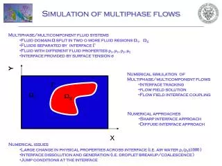
Secondary Phase Primary Phase Introduction • A phase is a class of matter with a definable boundary and a particular dynamic response to the surrounding flow/potential field. • Phases are generally identified by solid, liquid or gaseous states of matter but can also refer to other forms: • Materials with different chemical properties but in the same state or phase (i.e. liquid-liquid, such as, oil-water) • The fluid system is defined by a primary and multiple secondary phases. • One of the phases is considered continuous (primary) • The others (secondary) are considered to be dispersed within the continuous phase. • There may be several secondary phase denoting particles with different sizes • In contrast, multi-component flow (species transport) refers to flow that can be characterized by a single velocity and temperature field for all species.
Choosing a Multiphase Model • In order to select the appropriate model, users must know a priori the characteristics of the flow in terms of the following: • Flow regime • Particulate (bubbles, droplets or solid particles in continuous phase) • Stratified (fluids separated by interface with length scale comparable to domain length scale) • Multiphase turbulence modeling • For particulate flow, one can estimate • Particle volume loading • Stokes number
Slug Flow Bubbly, Droplet, or Particle-Laden Flow Stratified / Free- Surface Flow Pneumatic Transport, Hydrotransport, or Slurry Flow Sedimentation Fluidized Bed Multiphase Flow Regimes • Bubbly flow – Discrete gaseous bubbles in a continuous fluid, e.g. absorbers, evaporators, sparging devices. • Droplet flow – Discrete fluid droplets in a continuous gas, e.g. atomizers, combustors • Slug flow – Large bubbles in a continuous liquid • Stratified / free-surface flow – Immiscible fluids separated by a clearly defined interface, e.g. free-surface flow • Particle-laden flow – Discrete solid particles in a continuous fluid, e.g. cyclone separators, air classifiers, dust collectors, dust-laden environmental flows • Fluidized beds – Fluidized bed reactors • Slurry flow – Particle flow in liquids, solids suspension, sedimentation, and hydro-transport Gas/Liquid Liquid/Liquid Gas / Solid Liquid / Solid
Volume and Particulate Loading • Volume loading – dilute or dense • Refers to the volume fraction of secondary phase(s) • For dilute loading (< 10%), the average inter-particle distance is around twice the particle diameter. Thus, interactions among particles can be neglected. • Particulate loading – ratio of dispersed and continuous phase inertias
Turbulence Modeling in Multiphase Flows • Turbulence modeling with multiphase flows is challenging. • Presently, single-phase turbulence models (such as k–ε or RSM) are used to model turbulence in the primary phase only. • Turbulence equations may contain additional terms to account for turbulence modification by secondary phase(s). • If phases are separated and the density ratio is of order 1 or if the particle volume fraction is low (< 10%), then a single-phase model can be used to represent the mixture. • In other cases, either single phase models are still used or “particle-presence-modified” models are used.
Stokes Number • For systems with intermediate particulate loading, the Stokes number provides a guidance for selecting the most appropriate model. • The Stokes number, St, is the ratio of the particle (i.e. dispersed phase) relaxation time (τd) to the characteristic time scale of the flow (τc). where and . • D and U are the characteristic length and velocity scales of the problem. • For St << 1, the particles will closely follow the flow field. • For St > 1, the particles move independently of the flow field.
Phases as Mixtures of Species • In all multiphase models within FLUENT, any phase can be composed of either a single material or a mixture of species. • Material definition of phase mixtures is the same as in single phase flows. • It is possible to model heterogeneous reactions (reactions where the reactants and products belong to different phases). • This means that heterogeneous reactions will lead to interfacial mass transfer.
Multiphase Models in FLUENT Define Models Multiphase… • Models suited for particulate flows • Discrete Phase Model (DPM) • Mixture Model • Eulerian Multiphase Flow Model • Models suited for stratified flows • Volume of Fluid Model (VOF) Define Phases…
Discrete Phase Model (DPM) • Trajectories of particles/droplets/bubbles are computed in a Lagrangian frame. • Particles can exchange heat, mass, and momentum with the continuous gas phase. • Each trajectory represents a group of particles of the same initial properties. • Particle-particle interactions are neglected. • Turbulent dispersion can be modeled using either stochastic tracking or a “particle cloud” model. • Numerous sub-modeling capabilities are available: • Heating/cooling of the discrete phase • Vaporization and boiling of liquid droplets • Volatile evolution and char combustion for combusting particles • Droplet breakup and coalescence using spray models • Erosion/Accretion
Applicability of DPM • Flow regime: Bubbly flow, droplet flow, particle-laden flow • Volume loading: Must be dilute (volume fraction < 12%) • Particulate Loading: Low to moderate • Turbulence modeling: Weak to strong coupling between phases • Stokes Number: All ranges of Stokes number • Application examples • Cyclones • Spray dryers • Particle separation and classification • Aerosol dispersion • Liquid fuel • Coal combustion
DPM Example – Spray Drier Simulation Air and methane inlets • Spray drying involves the transformation of a liquid spray into dry powder in a heated chamber. The flow, heat, and mass transfer are simulated using the FLUENT DPM. • CFD simulation plays a very important role in optimizing the various parameters for the spray dryer. Centerline for particle injections Outlet Path Lines Indicating the Gas Flow Field
Spray Dryer Simulation (2) Contours of Evaporated Water Initial particle Diameter: 2 mm 1.1 mm 0.2 mm Stochastic Particle Trajectories for Different Initial Diameters
The Eulerian Multiphase Model • The Eulerian multiphase model is a result of averaging of NS equations over the volume including arbitrary particles + continuous phase. • The result is a set of conservation equations for each phase (continuous phase + N particle “media”). • Both phases coexist simultaneously: conservation equations for each phase contain single-phase terms (pressure gradient, thermal conduction etc.) + interfacial terms. • Interfacial terms express interfacial momentum (drag), heat and mass exchange. These are nonlinearly proportional to degree of mechanical (velocity difference between phases), thermal (temperature difference). Hence equations are harder to converge. • Add-on models (turbulence etc.) are available.
The Granular Option in the Eulerian Model • Granular flows occur when high concentration of solid particles is present. This leads to high frequency of interparticle collisions. • Particles are assumed to behave similar to a dense cloud of colliding molecules. Molecular cloud theory is applied to the particle phase. • Application of this theory leads to appearance of additional stresses in momentum equations for continuous and particle phases • These stresses (granular “viscosity”, “pressure” etc.) are determined by intensity of particle velocity fluctuations • Kinetic energy associated with particle velocity fluctuations is represented by a “pseudo-thermal” or granular temperature • Inelasticity of the granular phase is taken into account
Applicability of Eulerian model • Flow regime Bubbly flow, droplet flow, slurry flow,fluidized beds, particle-laden flow • Volume loading Dilute to dense • Particulate loading Low to high • Turbulence modeling Weak to strong coupling between phases • Stokes number All ranges • Application examples • High particle loading flows • Slurry flows • Sedimentation • Hydrotransport • Fluidized beds • Risers • Packed bed reactors
Eulerian Example – 3D Bubble Column z = 20 cm z =15 cm z =10 cm z =5 cm Iso-Surface of Gas Volume Fraction = 0.175 Liquid Velocity Vectors
Eulerian Example – Circulating Fluidized Bed Contours of Solid Volume Fraction
The Mixture Model Courtesy of Fuller Company
The Mixture Model • The mixture model is a simplified Eulerian approach for modeling n-phase flows. • The simplification is based on the assumption that the Stokes number is small (particle and primary fluid velocity is nearly equal in both magnitude and direction). • Solves the mixture momentum equation (for mass-averaged mixture velocity) and prescribes relative velocities to describe the dispersed phases. • Interphase exchange terms depend on relative (slip) velocities which are algebraically determined based on the assumption that St << 1. This means that phase separation cannot be modeled using the mixture model. • Turbulence and energy equations are also solved for the mixture if required. • Solves a volume fraction transport equation for each secondary phase. • A submodel for cavitation is available (see the Appendix for details).
Applicability of Mixture model • Flow regime: Bubbly, droplet, and slurry flows • Volume loading: Dilute to moderately dense • Particulate Loading: Low to moderate • Turbulence modeling: Weak coupling between phases • Stokes Number: St << 1 • Application examples • Hydrocyclones • Bubble column reactors • Solid suspensions • Gas sparging
Mixture Model Example – Gas Sparging • The sparging of nitrogen gas into a stirred tank is simulated by the mixture multiphase model. The rotating impeller is simulated using the multiple reference frame (MRF) approach. • FLUENT simulation provided a good prediction on the gas-holdup of the agitation system. Contours of Gas Volume Fraction at t = 15 sec. Water Velocity Vectors on a Central Plane
The Volume of Fluid (VOF) Model • The VOF model is designed to track the position of the interface between two or more immiscible fluids. • Tracking is accomplished by solution of phase continuity equation – resulting volume fraction abrupt change points out the interface location. • A mixture fluid momentum equation is solved using mixture material properties. Thus the mixture fluid material properties experience jump across the interface. • Turbulence and energy equations are also solved for mixture fluid. • Surface tension and wall adhesion effects can be taken into account. • Phases can be compressible and be mixtures of species
vapor liquid vapor liquid Interface Interpolation Schemes • The standard interpolation schemes used in FLUENT are used to obtain the face fluxes whenever a cell is completely filled with one phase. • The schemes are: • Geometric Reconstruction • Default scheme, unsteady flow only, no numerical diffusion, sensitive to grid quality • Euler Explicit • Unsteady flow only, can be used on skewed cells numerical diffusion is inherent – use high order VOF discretization (HRIC, CICSAM) • Euler Implicit • Compatible with both steady and unsteady solvers, can be used on skewed cells numerical diffusion is inherent – use high order VOF discretization (HRIC, CICSAM) Actual interface shape Geo-reconstruct (piecewise linear) Scheme
Applicability of VOF model • Flow regime Slug flow, stratified/free-surface flow • Volume loading Dilute to dense • Particulate loading Low to high • Turbulence modeling Weak to moderate coupling between phases • Stokes number All ranges • Application examples • Large slug flows • Filling • Offshore separator sloshing • Boiling • Coating
VOF Example – Automobile Fuel Tank Sloshing • Sloshing (free surface movement) of liquid in an automotive fuel tank under various accelerating conditions is simulated by the VOF model in FLUENT. • Simulation shows the tank with internal baffles (at bottom) will keep the fuel intake orifice fully submerged at all times, while the intake orifice is out of the fuel at certain times for the tank without internal baffles (top). t= 2.05 sec Fuel Tank Without Baffles t= 1.05 sec Fuel Tank With Baffles
VOF Example – Horizontal Film Boiling Plots showing the rise of bubbles during the film boiling process (the contours of vapor volume fraction are shown in red)
Summary • Choose an appropriate model for your application based on flow regime, volume loading, particulate loading, turbulence, and Stokes number. • Use VOF for free surface and stratified flows. • Use the Eulerian granular model for high particle loading flows. • Consider the Stokes number in low to moderate particle loading flows. • For St > 1, the mixture model is not applicable. Instead, use either DPM or Eulerian. • For St 1, all models are applicable. Use the least CPU demanding model based on other requirements. • Strong coupling among phase equations solve better with reduced under-relaxation factors. • Users should understand the limitations and applicability of each model.
Discrete Phase Model (DPM) Setup Define Models Discrete Phase… Define Injections… Display Particle Tracks…
DPM Boundary Conditions • Escape • Trap • Reflect • Wall-jet
Mixture Model Equations • Solves one equation for continuity of the mixture • Solves for the transport of volume fraction of each secondary phase • Solves one equation for the momentum of the mixture • The mixture properties are defined as: Drift velocity
Mixture Model Setup (1) Define Models Multiphase… Define Phases…
Mixture Model Setup (2) • Boundary Conditions • Volume fraction defined for each secondary phase. • To define initial phase location, patch volume fractions after solution initialization.
Cavitation Submodel • The Cavitation model models the formation of bubbles when the local liquid pressure is below the vapor pressure. • The effect of non-condensable gases is included. • Mass conservation equation for the vapor phase includes vapor generation and condensation terms which depend on the sign of the difference between local pressure and vapor saturation pressure (corrected for on-condensable gas presence). • Generally used with the mixture model, incompatible with VOF. • Tutorial is available for learning the in-depth setup procedure.
Eulerian Multiphase Model Equations • Continuity: • Momentum for qth phase: • The inter-phase exchange forces are expressed as: In general: • Energy equation for the qth phase can be similarly formulated. Volume fraction for the qth phase transient convection pressure body shear interphase massexchange external, lift, andvirtual mass forces interphase forcesexchange Solids pressure term is included for granular model. Exchange coefficient
Eulerian Multiphase Model Equations • Multiphase species transport for species i belonging to mixture of qth phase • Homogeneous and heterogeneous reactions are setup the same as in single phase • Ansys The same species may belong to different phases without any relation between themselves Mass fraction of species i in qth phase homogeneous reaction convective transient diffusion heterogeneous reaction homogeneous production
Eulerian Model Setup Define Phases… Define Models Viscous…
Eulerian-Granular Model Setup • Granular option must be enabled when defining the secondary phases. • Granular properties require definition. • Phase interaction models appropriate for granular flows must be selected.
VOF Model Setup Define Models Multiphase… Define Phases… Define Operating Conditions… Operating Densityshould be set to that of lightest phase with body forces enabled.
Heterogeneous Reaction Setup Define Phases…
Mixture Domain Phase 2 Domain UDFs for Multiphase Applications 1 Domain ID = • When a multiphase model is enabled, storage for properties and variables is set aside for mixture as well as for individual phases. • Additional thread and domain data structures required. • In general the type of DEFINE macro determines which thread or domain (mixture or phase) gets passed to your UDF. • C_R(cell,thread) will return the mixture density if thread is the mixture thread or the phase densities if it is the phase thread. • Numerous macros exist for data retrieval. Mixture Thread Phase 1 Domain Phase 3 Domain 2 3 4 Interaction Domain 5 Phase Thread Domain ID