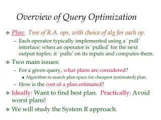
An Overview of Query Optimization
370 likes | 516 Views
An Overview of Query Optimization. Chapter 14. Query Evaluation. Problem : An SQL query is declarative – does not specify a query execution plan. A relational algebra expression is procedural – there is an associated query execution plan.

An Overview of Query Optimization
E N D
Presentation Transcript
An Overview of Query Optimization Chapter 14
Query Evaluation • Problem: An SQL query is declarative – does not specify a query execution plan. • A relational algebra expression is procedural – there is an associated query execution plan. • Solution: Convert SQL query to an equivalent relational algebra and evaluate it using the associated query execution plan. • But which equivalent expression is best?
Naive Conversion • SELECT DISTINCTTargetList • FROM R1, R2, …, RN • WHERE Condition • is equivalent to • TargetList(Condition (R1 R2 ... RN)) • but this may imply a very inefficient query execution plan. • Example: Name(Id=ProfId CrsCode=‘CS532’ (Professor Teaching)) • Result can be < 100 bytes • But if each relation is 50K then we end up computing an • intermediate result Professor Teaching of size 1G • before shrinking it down to just a few bytes. • Problem: Find an equivalent relational algebra expression that can be evaluated “efficiently”.
Query Optimizer • Uses heuristic algorithms to evaluate relational algebra expressions. This involves: • estimating the cost of a relational algebra expression • transforming one relational algebra expression to an equivalent one • choosing access paths for evaluating the subexpressions • Query optimizers do not “optimize” – just try to find “reasonably good” evaluation strategies
Equivalence Preserving Transformations • To transform a relational expression into another equivalent expression we need transformation rules that preserve equivalence • Each transformation rule • Is provably correct (ie, does preserve equivalence) • Has a heuristic associated with it
Selection and Projection Rules • Break complex selection into simpler ones: • Cond1Cond2 (R) Cond1(Cond2 (R) ) • Break projection into stages: • attr (R) attr (attr (R)), if attr attr • Commute projection and selection: • attr (Cond(R)) Cond (attr (R)), if attr all attributes in Cond
Commutativity and Associativity of Join(and Cartesian Product as Special Case) • Join commutativity: R S S R • used to reduce cost of nested loop evaluation strategies (smaller relation should be in outer loop) • Join associativity: R (S T) (R S) T • used to reduce the size of intermediate relations in computation of multi-relational join – first compute the join that yields smaller intermediate result • N-way join has T(N) N! different evaluation plans • T(N) is the number of parenthesized expressions • N! is the number of permutations • Query optimizer cannot look at all plans (might take longer to find an optimal plan than to compute query brute-force). Hence it does not necessarily produce optimal plan
Pushing Selections and Projections • Cond (R S) R Cond S • Cond relates attributes of both R and S • Reduces size of intermediate relation since rows can be discarded sooner • Cond (R S) Cond (R) S • Cond involves only the attributes of R • Reduces size of intermediate relation since rows of R are discarded sooner • attr(R S) attr(attr (R) S), if attributes(R) attr attr • reduces the size of an operand of product
Equivalence Example • C1 C2 C3 (R S) C1(C2(C3(R S) ) ) C1(C2(R) C3(S) ) C2(R) C1C3(S) assuming C2 involves only attributes of R, C3 involves only attributes of S, and C1 relates attributes of R and S
Cost - Example 1 SELECT P.Name FROMProfessor P, Teaching T WHERE P.Id = T.ProfId -- join condition AND P. DeptId = ‘CS’ AND T.Semester = ‘F1994’ Name(DeptId=‘CS’ Semester=‘F1994’(ProfessorId=ProfIdTeaching)) Name DeptId=‘CS’ Semester=‘F1994’ Id=ProfId Master query execution plan (nothing pushed) ProfessorTeaching
Metadata on Tables (in system catalogue) • Professor (Id, Name, DeptId) • size: 200 pages, 1000 rows, 50 departments • indexes: clustered, 2-level B+tree on DeptId, hash on Id • Teaching (ProfId, CrsCode, Semester) • size: 1000 pages, 10,000 rows, 4 semesters • indexes: clustered, 2-level B+tree on Semester; hash on ProfId • Definition: Weight of an attribute – average number of rows that have a particular value • weight of Id = 1 (it is a key) • weight of ProfId = 10 (10,000 classes/1000 professors)
Estimating Cost - Example 1 • Join - block-nested loops with 52 page buffer (50 pages – input for Professor, 1 page – input for Teaching, 1 – output page • Scanning Professor (outer loop): 200 page transfers, (4 iterations, 50 transfers each) • Finding matching rows in Teaching (inner loop): 1000 page transfers for each iteration of outer loop • 250 professors in each 50 page chunk * 10 matching Teaching tuples per professor = 2500 tuple fetches = 2500 page transfers for Teaching (Why?) • By sorting the record Ids of these tuples we can get away with only 1000 page transfers (Why?) • total cost = 200+4*1000 = 4200 page transfers
Estimating Cost - Example 1 (cont’d) • Selection and projection – scan rows of intermediate file, discard those that don’t satisfy selection, project on those that do, write result when output buffer is full. • Complete algorithm: • do join, write result to intermediate file on disk • read intermediate file, do select/project, write final result • Problem: unnecessary I/O
Pipelining • Solution: use pipelining: • join and select/project act as coroutines, operate as producer/consumer sharing a buffer in main memory. • When join fills buffer; select/project filters it and outputs result • Process is repeated until select/project has processed last output from join • Performing select/project adds no additional cost join Intermediate result select/project output final result buffer
Estimating Cost - Example 1 (cont’d) • Total cost: 4200 + (cost of outputting final result) • We will disregard the cost of outputting final result in comparing with other query evaluation strategies, since this will be same for all
Cost Example 2 SELECT P.Name FROMProfessor P, Teaching T WHERE P.Id = T.ProfIdAND P. DeptId = ‘CS’ AND T.Semester = ‘F1994’ Name(Semester=‘F1994’ (DeptId=‘CS’ (Professor) Id=ProfIdTeaching)) Name Semester=‘F1994’ DeptId=‘CS’ ProfessorTeaching Partially pushed plan:selection pushed toProfessor Id=ProfId
Cost Example 2 -- selection • Compute DeptId=‘CS’(Professor) (to reduce size of one join table) using clustered, 2-level B+ tree on DeptId. • 50 departments and 1000 professors; hence weight of DeptId is 20 (roughly 20 CS professors). These rows are in ~4 consecutive pages in Professor. • Cost = 4 (to get rows) + 2 (to search index) = 6 • keep resulting 4 pages in memory and pipe to next step clustered index on DeptId rows of Professor
Cost Example 2 -- join • Index-nested loops join using hash index on ProfId of Teaching and looping on the selected professors (computed on previous slide) • Since selection on Semester was not pushed, hash index on ProfId of Teaching can be used • Note: if selection on Semester were pushed, the index on ProfId would have been lost – an advantage of not using a fully pushed query execution plan
Cost Example 2 – join (cont’d) • Each professor matches ~10 Teaching rows. Since 20 CS professors, hence 200 teaching records. • All index entries for a particular ProfId are in same bucket. Assume ~1.2 I/Os to get a bucket. • Cost = 1.2 20 (to fetch index entries for 20 CS professors) + 200 (to fetch Teaching rows, since hash index is unclustered) = 224 Teaching 1.2 20 10 hash ProfId
Cost Example 2 – select/project • Pipe result of join to select (on Semester) and project (on Name) at no I/O cost • Cost of output same as for Example 1 • Total cost: 6 (select on Professor) + 224 (join) = 230 • Comparison: 4200 (example 1) vs. 230 (example 2) !!!
Estimating Output Size • It is important to estimate the size of the output of a relational expression – size serves as input to the next stage and affects the choice of how the next stage will be evaluated. • Size estimation uses the following measures on a particular instance of R: • Tuples(R): number of tuples • Blocks(R): number of blocks • Values(R.A): number of distinct values of A • MaxVal(R.A): maximum value of A • MinVal(R.A): minimum value of A
Blocks (result set) Blocks(R1) ... Blocks(Rn) Estimating Output Size • For the query: • Reduction factor is • Estimates by how much query result is smaller than input SELECTTargetList FROM R1, R2, …, Rn WHERECondition
Estimation of Reduction Factor • Assume that reduction factors due to target list and query condition are independent • Thus: reduction(Query) = reduction(TargetList) reduction(Condition)
1 Values(R.A) 1 max(Values(Ri.A), Values(Rj.B)) MaxVal(Ri.A) – val MaxVal(Ri.A) – MinVal(Ri.A) Reduction Due to Simple Condition • reduction (Ri.A=val) = • reduction (Ri.A=Rj.B) = • Assume that values are uniformly distributed, Tuples(Ri) < Tuples(Rj), and every row of Ri matches a row of Rj . Thenthe number of tuples that satisfy Condition is: • reduction (Ri.A > val) = • Values(Ri.A) (Tuples(Ri.A)/Values(Ri.A)) • (Tuples(Rj.A)/Values(Rj.A))
Reduction Due to Complex Condition • reduction(Cond1ANDCond2) = reduction(Cond1) reduction(Cond2) • reduction(Cond1ORCond2) = min(1, reduction(Cond1) + reduction(Cond2))
number-of-attributes (TargetList) inumber-of-attributes (Ri) Reduction Due to TargetList • reduction(TargetList) =
Estimating Weight of Attribute weight(R.A) = Tuples(R) reduction(R.A=value)
Choosing Query Execution Plan • Step 1: Choose a logical plan • Step 2: Reduce search space • Step 3: Use a heuristic search to further reduce complexity
Step 1: Choosing a Logical Plan • Involves choosing a query tree, which indicates the order in which algebraic operations are applied • Heuristic: Pushed trees are good, but sometimes “nearly fully pushed” trees are better due to indexing (as we saw in the example) • So: Take the initial “master plan” tree and produce a fully pushed tree plus several nearly fully pushed trees.
Step 2: Reduce Search Space • Deal with associativity of binary operators (join, union, …) D A B C D C A B C D Logical query execution plan A B Equivalent query tree Equivalent left deep query tree
Step 2 (cont’d) • Two issues: • Choose a particular shape of a tree (like in the previous slide) • Equals the number of ways to parenthesize N-way join – grows very rapidly • Choose a particular permutation of the leaves • E.g., 4! permutations of the leaves A, B, C, D
P1 P2 P3 A B X C Y D X Y Step 2: Dealing With Associativity • Too many trees to evaluate: settle on a particular shape: left-deep tree. • Used because it allows pipelining: • Property: once a row of X has been output by P1, it need not be output again (but C may have to be processed several times in P2 for successive portions of X) • Advantage: none of the intermediate relations (X, Y) have to be completely materialized and saved on disk. • Important if one such relation is very large, but the final result is small
Step 2: Dealing with Associativity • consider the alternative: if we use the association ((A B) (C D)) A B P1 P2 Each row of X must be processed against all of Y. Hence all of Y (can be very large) must be stored in P3, or P2 has to recompute it several times. X X Y C D Y P3
Step 3: Heuristic Search • The choice of left-deep trees still leaves open too many options (N! permutations): • (((A B) C) D), • (((C A) D) B), ….. • A heuristic (often dynamic programming based) algorithm is used to get a ‘good’ plan
Step 3: Dynamic Programming Algorithm • Just an idea – see book for details • To compute a join of E1, E2, …, EN in a left-deep manner: • Start with 1-relation expressions (can involve , ) • Choose the best and “nearly best” plans for each (a plan is considered nearly best if its out put has some “interesting” form, e.g., is sorted) • Combine these 1-relation plans into 2-relation expressions. Retain only the best and nearly best 2-relation plans • Do same for 3-relation expressions, etc.
Index-Only Queries • A B+ tree index with search key attributes A1, A2, …, Anhas stored in it the values of these attributes for each row in the table. • Queries involving a prefix of the attribute list A1, A2, .., Ancan be satisfied using only the index – no access to the actual table is required. • Example: Transcript has a clustered B+ tree index on StudId. A frequently asked query is one that requests all grades for a given CrsCode. • Problem: Already have a clustered index on StudId – cannot create another one (on CrsCode) • Solution: Create an unclustered index on (CrsCode, Grade) • Keep in mind, however, the overhead in maintaining extra indices