Download

1 / 22
240 likes | 369 Views
This lecture by Professor Ronald L. Carter delves into the complexities of semiconductor device modeling and characterization. It focuses on low and high-level injection effects, parameters extraction, and junction capacitance estimation. Key points include the relationship between current and voltage, how to interpret data plots, and the significance of parameters like Rs, IS, and Neff in device performance. The lecture provides essential insights for advanced students aiming to understand semiconductor behaviors and optimize device efficiency.

E N D
EE5342 – Semiconductor Device Modeling and CharacterizationLecture 10 - Spring 2005 Professor Ronald L. Carter ronc@uta.edu http://www.uta.edu/ronc/
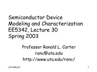
Vext-Va=iD*Rs low level injection ln iD ln(IKF) Effect ofRs ln[(IS*IKF) 1/2] Effect of high level injection ln(ISR) Data ln(IS) vD= Vext recomb. current VKF
Interpreting a plotof log(iD) vs. Vd In the region where iD ~ ISeff(exp (Vd/(NeffVt)) - 1) For N = 1 and Vt = 25.852 mV, the slope of the plot of log(iD) vs. Vd is evaluated as {dlog(iD)/dVd} = log (e)/(NVt) = 16.799 decades/V = 1decade/59.526mV
Static Model Eqns.Parameter Extraction In the region where iD ~ ISeffexp (Vd/(NeffVt) ) {diD/dVd}/iD = d[ln(iD)]/dVd = 1/(NVt) so N ~ {dVd/d[ln(iD)]}/Vt Neff, and ln(IS) ~ ln(iD) - Vd/(NVt) ln(ISeff). Note: iD, Vt, etc., are normalized to 1A, 1V, resp.
Hints for RS and NFparameter extraction In the region where vD > VKF. Defining vD = vDext - iD*RS and IHLI = [ISIKF]1/2. iD = IHLIexp (vD/2NVt) + ISRexp (vD/NRVt) diD/diD = 1 (iD/2NVt)(dvDext/diD - RS) + … Thus, for vD > VKF (highest voltages only) • plot iD-1vs. (dvDext/diD) to get a line with • slope = (2NVt)-1, intercept = - RS/(2NVt)
Application of RS tolower current data In the region where vD < VKF. We still have vD = vDext - iD*RS and since. iD = ISexp (vD/NVt) + ISRexp (vD/NRVt) • Try applying the derivatives for methods described to the variables iD and vD (using RS and vDext). • You also might try comparing the N value from the regular N extraction procedure to the value from the previous slide.
Estimating Junction Capacitance Parameters • Following L29 – EE 5340 Fall 2003 • If CJ = CJO {1 – Va/VJ}-M • Define y {d[ln(CJ)]/dV}-1 • A plot of y = yi vs. Va = vi has slope = -1/M, and intercept = VJ/MF
Derivatives Defined The central derivative is defined as (following Lecture 14 and 11) yi,Central = (vi+1 – vi-1)/(lnCi+1 – lnCi-1), with vi = (vi+1 + vi-1)/2 Equation A1.1 The Forward derivative (as applied to the theory in L11 and L14) is defined in this case as yi,Forward = (vi+1 – vi)/(lnCi+1 – lnCi), with vi,eff = (vi+1 + vi-1)/2 Equation A1.2
Data calculations Table A1.1. Calculations of yi and vi for the Central and Forward derivatives for the data in Table 1. The yi and vi are defined in Equations A1.1 and A1.2.
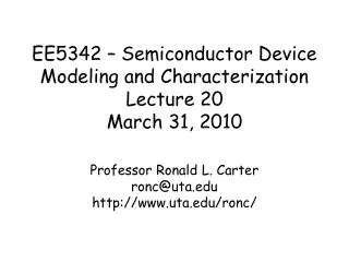
y vs. Va plots Figure A1.3. The yi and vi values from the theory in L11 and L14 with associa-ted trend lines and slope, intercept and R^2 values.
It is clear the Central derivative gives the more reliable data as the R^2 value is larger. M is the reciprocal of the magnitude of the slope obtained by a least squares fit (linear) plot of yi vs. Vi VJ is the horizontal axis intercept (computed as the vertical axis intercept divided by the slope) Cj0 is the vertical axis intercept of a least squares fit of Cj-1/M vs. V (must use the value of V for which the Cj was computed). The computations will be shown later. The results of plotting Cj-1/M vs. V for the M value quoted below are shown in Figure A1.4 Comments on thedata interpretation
M = 1/2.551 = 0.392 (the data were generated using M = 0.389, thus we have a 0.77% error). VJ = yi(vi=0)/slope =1.6326/2.551 = 0.640 (the data were generated using fi = 0.648, thus we have a 1.24% error). Cj0 = 1.539E30^-.392 = 1.467 pF (the data were generated using Cj0 = 1.68 pF, thus we have a 12.6% error) Calculating theparameters
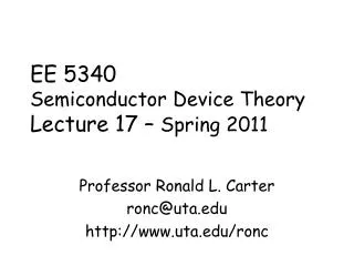
Linearized C-V plot Figure A1.4. A plot of the data for Cj^-1/M vs. Va using the M value determined for this data (M = 0.392).
Doping Profile The data were equal-ly spaced (DV=0.1V), the central differ-ence was used, for -7.4V ≤ V ≤ 0.4V, which for Cj = e/x, corresponds to a range of 2.81E-5 cm ≤ x ≤ 8.99E-5 cm. These data are shown. The trend line is also shown for a linear fit. Since R^2 = 1.000, a linear N(x) relationship can be assumed.
SPICE Diode Capacitance Pars.1 PARAMETER definition and units default value TT transit time sec 0.0 CJO zero-bias p-n capacitance farad 0.0 M p-n grading coefficient 0.5 FC forward-bias depletion capacitance coeff 0.5 VJ p-n potential volt 1.0
SPICE Diode Capacitance Eqns.1 Cd = Ct + area·Cj Ct = transit time capacitance = TT·Gd Gd = DC conductance = area * d (Inrm Kinj + Irec Kgen)/dVd Kinj = high-injection factor Cj = junction capacitance IF: Vd < FC·VJ Cj = CJO*(1-Vd/VJ)^(-M) IF: Vd > FC·VJ Cj = CJO*(1-FC)^(-1-M)·(1-FC·(1+M)+M·Vd/VJ)
Junction Capacitance • A plot of [Cj]-1/Mvs. Vd hasSlope = -[(CJO)1/M/VJ]-1 vertical axis intercept = [CJO]-2 horizontal axis intercept = VJ Cj-1/M CJO-1/M Vd VJ
Junction Width and Debye Length • LD estimates the transition length of a step-junction DR (concentrations Na and Nd with Neff = NaNd/(Na +Nd)). Thus, • For Va=0, & 1E13 <Na,Nd< 1E19 cm-3 13% <d< 28% => DA is OK
Junction CapacitanceAdapted from Figure 1-16 in Text2 Cj = CJO/(1-Vd/VJ)^M Cj = CJO/(1-FC)^(1+M)* (1-FC·(1+M)+M·Vd/VJ) FC*VJ VJ