Overview of Biomedical Engineering Measurement Systems and Applications
310 likes | 451 Views
This chapter delves into the multifaceted domains of biomedical engineering, highlighting key systems and methodologies used in the field. It covers essential topics such as bioinstrumentation, biomechanics, biosignals, and clinical engineering, alongside practical applications in agriculture, medicine, and veterinary science. Through tables and figures, the text illustrates the scientific method, measurement systems, and the role of clinicians in effective healthcare settings. The integration of biosystems and cell engineering highlights the importance of calibration, accuracy, and precision in biomedical instrumentation.

Overview of Biomedical Engineering Measurement Systems and Applications
E N D
Presentation Transcript
Chapter 1 Measurement Systems
Bioinstrumentation • Biomaterials • Biomechanics • Biosignals • Biosystems • Biotransport • Cellular engineering • Clinical engineering • Tissue engineering • Rehabilitation engineering Table 1.1 Biomedical engineers work in a variety of fields.
Agriculture - Soil monitoring • Botany - Measurements of metabolism • Genetics - Human genome project • Medicine - Anesthesiology • Microbiology - Tissue analysis • Pharmacology - Chemical reaction monitoring • Veterinary science - Neutering of animals • Zoology - Organ modeling Table 1.2 Biomedical engineers work in a variety of disciplines. One example of instrumentation is listed for each discipline.
Table 1.3 Biomedical engineers may work in a variety of environments.
Figure 1.1 In the scientific method, a hypothesis is tested by experiment to determine its validity.
Figure 1.2 The physician obtains the history, examines the patient, performs tests to determine the diagnosis and prescribes treatment.
Figure 1.3 A typical measurement system uses sensors to measure the variable, has signal processing and display, and may provide feedback.
(a) (b) Figure 1.4 (a) Without the clinician, the patient may be operating in an ineffective closed loop system. (b) The clinician provides knowledge to provide an effective closed loop system.
Figure 1.5 In some situations, a patient may monitor vital signs and notify a clinician if abnormalities occur.
Table 1.5 Sensor specifications for a blood pressure sensor are determined by a committee composed of individuals from academia, industry, hospitals, and government.
Figure 1.6 A hysteresis loop. The output curve obtained when increasing the measurand is different from the output obtained when decreasing the measurand.
(a) (b) Figure 1.7 (a) A low-sensitivity sensor has low gain. (b) A high sensitivity sensor has high gain.
(a) (b) Figure 1.8 (a) Analog signals can have any amplitude value. (b) Digital signals have a limited number of amplitude values.
Table 1.6 Specification values for an electrocardiograph are agreed upon by a committee.
(b) (a) Figure 1.9 (a) An input signal which exceeds the dynamic range. (b) The resulting amplified signal is saturated at 1 V.
(b) (a) Figure 1.10 (a) An input signal without dc offset. (b) An input signal with dc offset.
(a) (b) Figure 1.12 (a) A linear system fits the equation y = mx + b. Note that all variables are italic. (b) A nonlinear system does not fit a straight line.
(a) (b) Figure 1.13 (a) Continuous signals have values at every instant of time. (b) Discrete-time signals are sampled periodically and do not provide values between these sampling times.
(a) (b) Figure 1.14 (a) Signals without noise are uncorrupted. (b) Interference superimposed on signals causes error. Frequency filters can be used to reduce noise and interference.
(b) (c) (a) Figure 1.15 (a) Original waveform. (b) An interfering input may shift the baseline. (c) A modifying input may change the gain.
(a) (b) Figure 1.16 Data points with (a) low precision and (b) high precision.
(a) (b) Figure 1.17 Data points with (a) low accuracy and (b) high accuracy.
(a) (b) Figure 1.18 (a) The one-point calibration may miss nonlinearity. (b) The two-point calibration may also miss nonlinearity.
Figure 1.19 For the normal distribution, 68% of the data lies within ±1 standard deviation. By measuring samples and averaging, we obtain the estimated mean , which has a smaller standard deviation sx. is the tail probability that xs does not differ from by more than .
Table 1.9 Equivalent table of Table 1.8 for results relating to a condition or disease.
Figure 1.21 The test result threshold is set to minimize false positives and false negatives.