Download

1 / 127
1.28k likes | 1.56k Views
One Pass Algorithm Presented By: Pradhyuman raol ID : 114. Instructor: Dr T.Y. LIN. Agenda . One Pass algorithm Tuple-at-a-Time Unary Operators Binary Operations. One-Pass Algorithms . One Pass Algorithm: Some methods involve reading the data only once from disk.

E N D
One Pass Algorithm Presented By: Pradhyuman raol ID : 114 Instructor: Dr T.Y. LIN
Agenda • One Pass algorithm • Tuple-at-a-Time • Unary Operators • Binary Operations
One-Pass Algorithms • One Pass Algorithm: • Some methods involve reading the data only once from disk. • They work only when at least one of the arguments of the operation fits in main memory.
Tuple-at-a-Time • We read the blocks of R one at a time into an input buffer, perform the operation on the tuple, and more the selected tuples or the projected tuples to the output buffer. • Examples: Selection & Projection
Tuple at a time Diagram R Unary operator Input buffer Output buffer
Unary Operators • The unary operations that apply to relations as a whole, rather than to one tuple at a time. • Duplicate Elimination d(R) :Check whether that tuple is already there or not. M= Main memory B(d(R))= Size of Relation R Assumption: B(d(R)) <= M
Unary Operators • Grouping : A grouping operation gives us zero or more grouping attributes and presumably one or more accumulated value or values for each aggregation. • Min or Max • Count • Sum • Average
Binary Operations • Set Union • Set Intersection • Set Difference • Bag Intersection • Bag Difference • Product • Natural join
Nested Loops Joins Book Section of chapter 15.3 Submitted to : Prof. Dr. T.Y. LIN Submitted by: Saurabh Vishal
Topic to be covered • Tuple-Based Nested-Loop Join • An Iterator for Tuple-Based Nested-Loop Join • A Block-Based Nested-Loop Join Algorithm • Analysis of Nested-Loop Join
15.3.1 Tuple-Based Nested-Loop Join • The simplest variation of nested-loop join has loops that range over individual tuples of the relations involved. In this algorithm, which we call tuple-based nested-loop join, we compute the join as follows R S
Continued • For each tuple s in S DO For each tuple r in R Do if r and s join to make a tuple t THEN output t; • If we are careless about how the buffer the blocks of relations R and S, then this algorithm could require as many as T(R)T(S) disk .there are many situations where this algorithm can be modified to have much lower cost.
Continued • One case is when we can use an index on the join attribute or attributes of R to find the tuples of R that match a given tuple of S, without having to read the entire relation R. • The second improvement looks much more carefully at the way tuples of R and S are divided among blocks, and uses as much of the memory as it can to reduce the number of disk I/O's as we go through the inner loop. We shall consider this block-based version of nested-loop join.
15.3.2 An Iterator for Tuple-Based Nested-Loop Join • Open() { • R.Open(); • S.open(); • A:=S.getnext(); } GetNext() { Repeat { r:= R.Getnext(); IF(r= Not found) {/* R is exhausted for the current s*/ R.close(); s:=S.Getnext();
IF( s= Not found) RETURN Not Found; /* both R & S are exhausted*/ R.Close(); r:= R.Getnext(); } } until ( r and s join) RETURN the join of r and s; } Close() { R.close (); S.close (); }
15.3.3 A Block-Based Nested-Loop Join Algorithm We can Improve Nested loop Join by compute R |><| S. • Organizing access to both argument relations by blocks. • Using as much main memory as we can to store tuples belonging to the relation S, the relation of the outer loop.
The nested-loop join algorithm FOR each chunk of M-1 blocks of S DO BEGIN read these blocks into main-memory buffers; organize their tuples into a search structure whose search key is the common attributes of R and S; FOR each block b of R DO BEGIN read b into main memory; FOR each tuple t of b DO BEGIN find the tuples of S in main memory that join with t ; output the join of t with each of these tuples; END ; END ; END ;
15.3.4 Analysis of Nested-Loop Join Assuming S is the smaller relation, the number of chunks or iterations of outer loop is B(S)/(M - 1). At each iteration, we read hf - 1 blocks of S and B(R) blocks of R. The number of disk I/O's is thus B(S)/M-1(M-1+B(R)) or B(S)+B(S)B(R)/M-1
Continued Assuming all of M, B(S), and B(R) are large, but M is the smallest of these, an approximation to the above formula is B(S)B(R)/M. That is, cost is proportional to the product of the sizes of the two relations, divided by the amount of available main memory.
Example • B(R) = 1000, B(S) = 500, M = 101 • Important Aside: 101 buffer blocks is not as unrealistic as it sounds. There may be many queries at the same time, competing for main memory buffers. • Outer loop iterates 5 times • At each iteration we read M-1 (i.e. 100) blocks of S and all of R (i.e. 1000) blocks. • Total time: 5*(100 + 1000) = 5500 I/O’s • Question: What if we reversed the roles of R and S? • We would iterate 10 times, and in each we would read 100+500 blocks, for a total of 6000 I/O’s. • Compare with one-pass join, if it could be done! • We would need 1500 disk I/O’s if B(S) M-1
Continued……. • The cost of the nested-loop join is not much greater than the cost of a one-pass join, which is 1500 disk 110's for this example. In fact.if B(S) 5 lZI - 1, the nested-loop join becomes identical to the one-pass join algorithm of Section 15.2.3 • Nested-loop join is generally not the most efficient join algorithm.
Summary of the topic In This topic we have learned about how the nested tuple Loop join are used in database using query execution and what is the process for that.
Presentation Topic 18.7 of Book Tree Protocol Submitted to: Prof. Dr. T.Y.LIN Submitted By :Saurabh Vishal
Topic’s That Should be covered in This Presentation • Motivation for Tree-Based Locking • Rules for Access to Tree-Structured Data • Why the Tree Protocol Works
Introduction • Tree structures that are formed by the link pattern of the elements themselves. Database are the disjoint pieces of data, but the only way to get to Node is through its parent. • B trees are best example for this sort of data. • Knowing that we must traverse a particular path to an element give us some important freedom to manage locks differently from two phase locking approaches.
Tree Based Locking • B tree index in a system that treats individual nodes( i.e. blocks) as lockable database elements. The Node Is the right level granularity. • We use a standard set of locks modes like shared,exculsive, and update locks and we use two phase locking
Rules for access Tree Structured Data • There are few restrictions in locks from the tree protocol. • We assume that that there are only one kind of lock. • Transaction is consider a legal and schedules as simple. • Expected restrictions by granting locks only when they do not conflict with locks already at a node, but there is no two phase locking requirement on transactions.
Why the tree protocol works. • A transaction's first lock may be at any node of the tree. • Subsequent locks may only be acquired if the transaction currently has a lock on the parent node. • Nodes may be unlocked at any time • A transaction may not relock a node on which it has released a lock, even if it still holds a lock on the node’s parent
Why the Tree Protocol works? • The Tree protocol forces a serial order on the transactions involved in a schedule. • Ti <sTj if in schedule S., the transaction Ti and Tj lock a node in common and Ti locks the node first.
Example • If precedence graph drawn from the precedence relations that we defined above has no cycles, then we claim that any topological order of transactions is an equivalent serial schedule. • For Example either ( T1,T2,T3) or (T3,T1,T2) is an equivalent serial schedule the reason for this serial order is that all the nodes are touched in the same order as they are originally scheduled.
If two transactions lock several elements in common, then they are all locked in same order. • I am Going to explain this with help of an example.
Continued…. • Now Consider an arbitrary set of transactions T1, T2;.. . . Tn,, that obey the tree protocol and lock some of the nodes of a tree according to schedule S. • First among those that lock, the root. they do also in same order. • If Ti locks the root before Tj, Then Ti locks every node in common with Tj does. That is Ti<sTj, But not Tj>sTi.
Concurrency Control by Timestamps Prepared By: Ronak Shah Professor :Dr. T. Y Lin ID: 116
Concurrency • Concurrency is a property of a systems in which several computations are executing and overlapping in time, and interacting with each other. Timestamp • Timestamp is a sequence of characters, denoting the date or time at which a certain event occurred. • Example of Timestamp: • 20-MAR-09 04.55.14.000000 PM • 06/20/2003 16:55:14:000000
Timestamping • We assign a timestamp to transaction and timestamp is usually presented in a consistent format, allowing for easy comparison of two different records and tracking progress over time; the practice of recording timestamps in a consistent manner along with the actual data is called timestamping.
Timestamps • To use timestamping as a concurrency-control method, the scheduler needs to assign to each transaction T a unique number, its timestamp TS(T). Here two approaches use to generating timestamps • Using system clock • Another approach is for the scheduler to maintain a counter. Each time when transaction starts the counter is incremented by 1 and new value become timestamp for transaction.
Whichever method we use to generate timestamp , the scheduler must maintain a table of currently active transaction and their timestamp. • To use timestamps as a concurrency-control method we need to associate with each database element x two timestamps and an additional bit. • RT(x) The read time of x. • WT(x) The write time of x. • C(x) The commit bit of x. which is true if and only if the most recent transaction to write x has already committed. The purpose of this bit is to avoid a situation of “Dirty Read”.
Physically Unrealizable Behaviors • Read too late Transaction T tries to read too late
Write too late Transaction T tries to write too late
Problem with dirty data T could perform a dirty read if it is reads X
A write is cancelled because of a write with a later timestamp, but the writer then aborts
Rules for timestamp based scheduling • Granting Request • Aborting T (if T would violate physical reality) and restarting T with a new timestamp (Rollback) • Delaying T and later deciding whether to abort T or to grant the request Scheduler’s Response to a T’s request for Read(X)/Write(X)
Rules • Request RT(X): • If TS(T) >= WT(X), the read is physically realizable • If C(X) is true, grant the request. If TS(T) > RT(X), set RT(X) := TS(T); otherwise do not change RT(X) • If C(X) is false, delay T until C(X) becomes true or the transaction that wrote X aborts • If TS(T) < WT(X), the read is physically unrealizable. Rollback T; abort T and restart it with a new, larger timestamp
Request WT(X): • If TS(T) >= RT(X) and TS(T) >= WT(X), the write is physically realizable and must be performed • Write the new value for X • Set WT(X) := TS(T), and • Set C(X) := false • If TS(T) >= RT(X), but TS(T) < WT(X), then the write is physically realizable, but there is already a later value in X. If C(X) is true, then ignore the write by T. If C(X) is false, delay T • If TS(T) < RT(X), then the write is physically unrealizable
Two-Pass Algorithms Based on Sorting Prepared By: Ronak Shah ID: 116