Download
1 / 1
20 likes | 160 Views
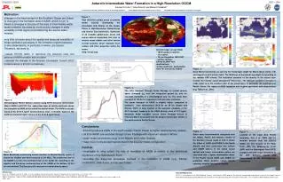
Antarctic Intermediate Water Formation in a High-Resolution OGCM. Antonio F.H. Fetter 1,2 , Victor Zlotnicki 1 , and Michael P. Schodlok 1,3. 1 Jet Propulsion Laboratory, California Institute of Technology, Pasadena 2 Universidade Federal de Pernambuco, Recife, Brazil

E N D
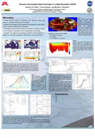
Antarctic Intermediate Water Formation in a High-Resolution OGCM Antonio F.H. Fetter1,2, Victor Zlotnicki1, and Michael P. Schodlok1,3 1Jet Propulsion Laboratory, California Institute of Technology, Pasadena 2 Universidade Federal de Pernambuco, Recife, Brazil 3JIFRESSE, University of California Los Angeles, Los Angeles Motivation: • assess ECCO2 ability to reproduce the observed rates and patterns of AAIW formation and circulation • estimate the changes in the Antarctic Circumpolar Current (ACC) frontal locations in ECCO2 and altimetry • investigate to what extent the rate of formation of AAIW is related to the meridional migrations of the Subantarctic Front (SAF) • elucidate the diapycnal processes involved in the formation of AAIW (e.g., Ekman contribution, eddy fluxes, and air-sea fluxes) Figure 1: High resolution global ocean circulation model ECCO2 (Estimating the Circulation and Climate of the Ocean, Phase II: High-Resolution Global-Ocean and Sea-Ice Data Synthesis). Syntheses of all available global-scale ocean and sea-ice data at resolutions that start to resolve ocean eddies and other narrow current systems, which transport heat, carbon, and other properties within the ocean (http://ecco2.org) ECCO2 model set up (CS84) • 18 km global resolution • 50 z-layers • 16 yrs integration 1992-2007 Figure 3: Saliniity section Antarctic Intermediate Water (AAIW) in ECCO2. The subsurface layer of salinity minimum shows the formation of AAIW at the end of the austral winter. The AAIW is usually found at the 27-27.4 kg/m3 neutral density class. In ECCO2, however, the AAIW is located at higher values, in the 27-27.8 kg/m3 class.4 (a) Figure. 2: Deep Winter Convection as seen by the mixed layer depth for March (boral winter, left) and August (austral winter, right). The thickness of the mixed layer depth is according to the models KPP criteria. The latitudinal zonation of the density in the mixed layer reveals the intense ocean-atmosphere interaction. The densest southern hemisphere mode water is in the southern part of the mixed layer, in particular the south-eastern Pacific Ocean, the region of AAIW formation and in good agreement with observations (e.g. Talley et al., 200x). Figure. 5: The ACC transport through Drake Passage in neutral density space averaged over the integration period (a), and the seasonal variability of a climatological year (b). The mean ACC transport of 145 Sv is in agreement with previous estimates. The mean transport of AAIW is slightly higher compared to estimates from observations (34.8 Sv vs 28 Sv; Sloyan and Rintoul, 2001). A large fraction of the seasonal variability of the ACC transport happens in the AAIW density class of 27.4 kg/m3. Maximum AAIW transport across Drake Passage occurs in February/March associated with the deepest mixed layer depths in the south eastern Pacific Ocean. Figure. 4: Mean Meridional overturning stream function in Neutral Density space. It shows the shallow and deep branches of the MOC. The southward flow of the NADW (~12 Sv), the northward flow of the AAIW, the upwelling at the equator and the dense northward flow of the AABW at the bottom (12 Sv) are well defined. The Deacon cell is present in neutral density space. (b) Conclusions: • A • B • C • D Fig. 6: Meridional overturning stream function in Neutral Density space. Fig. 6: Location of the Subantarctic Front according to Orsi et al, 1995 and ECCo2 The location of the PF, SAF and STF in ECCO2 compare well with the estimates of Orsi et al. (1995). The figure also shows the water mass transformation integrated over the Indian, Pacific and Atlantic oceans, south of 30S. It shows the inflow of AAIW and NADW in the South Atlantic and their conversion into surface and AABW waters. The Indian Ocean converts bottom and heavy intermediate water into a lighter intermediate water. The Pacific produces AAIW and AABW.