Download
1 / 25
250 likes | 444 Views
Serial Correlation and the Housing price function. Aka “Autocorrelation”. More on House prices. We return to the house price function to illustrate the issue of serial correlation It turns out that OLS may NOT give us the best estimate of the price function

E N D
Serial Correlation and the Housing price function Aka “Autocorrelation”
More on House prices • We return to the house price function to illustrate the issue of serial correlation • It turns out that OLS may NOT give us the best estimate of the price function • The reason is that one of the assumptions of the GM theorem is probably violated in the consumption model • The data is probably serially correlated • E[utut-1] ≠ 0
The Issue • In time series we can think of the residual as representing an economic shock • This is literally true in a statistical sense but may also be true in an economic sense • If the residual really is an economic shock it is a sort of omitted variable • It is likely that the effect of the shock persist across calender time periods • Think of the current economic situation: crisis will not stop on 31st of dec • Cant happen in cross section data
The Impact • This implies that the residuals will be correlated across time • Violates the GM theorem • Specifically if we estimate the model Yt=b1+b2Xt+ut • GM requires: • var[ut] =E[ut2]= 2(homoskedasticty) • E[utut-1] = 0 (no autocorrelation) • The second is likely violated in time series data
Characteristics of Serial Correlation • Systematic pattern exists in residuals • First order serial correlation:ut = ut-1 + vt • effect from error in previous period ut-1, • random error vtwhich satisfies the OLS assumptions • Think of what happens if rho is positive: • a positive shock tends to be followed by another positive shock • The shock persists • Aside: This is known as first order serial correlation. You can have serial correlation of higher order but we wont deal with it here. An example would be • ut= 1 ut-1 + 2 ut-2+ …….. + kut-k +vt
Serial Correlation vs Het • Systematic pattern exists in the residuals • Similar idea to heteroscedasticity but crucially different • Recall Het is a pattern in variance of residuals • Serial correlation is correlation between the draws from the same distribution • Think of the dice or roulette wheel example • Intuition: if random bit come from roll of dice then homo is with same dice and hetero is with different dice • Rolls of same dice for different people but rolls are linked • Note to confuse the issue: the two phenomena can occur together (GARCH) • We will treat them as separate • Evident in time series and not cross section because no natural ordering of data
Consequences • OLS is unbiased • OLS is consistent • OLS is no longer efficient • Variance formula used previously is incorrect • significance test, confidence intervals etc. cannot be used • Aside: a corrected formula can be used • Stata: regress y x, robust • We don’t bother with this because can do better with alternative estimator • Same consequences as Het – which can lead to confusion
Testing for AC • Plot of residuals against time • Stata: scatter u year • Plot residuals against lagged value • Scatter u L.u • Not a formal test but can give an idea of what's going on • Graphs are from housing data • Looks like there is positive serial correlation • Not surprising given the bubble
The Durbin Watson Test • Formal test of AC • Most complicated hypothesis test we have encountered • Wont work with all AC • Test requires • Testing for first order only • model must include intercept • model cannot include a lagged dependent variable (this is a big problem)
Formal Structure of the test • H0: =0 H1a: <0 H1b: >0, • Form the test statistic: Stata command: dwstat • Find the critical values from DW tables • N,K and SL • Each reading will produce two value: du and dL • Compare the test statistic and the critical values using the chart (over) • State Conclusion
Comments • The test statistic is (sort of) the coefficient of regression of residual on its lagged value • It is approximately equal to 2(1-rho)
This explains the boundaries on the chart • We have this slightly weird set-up because we don’t actually know the critical values for this test with certainty • All we know is min and max values for the true critical value: du and dL • This hypothesis test is unusual in that there is a zone of indecision where the test produces no result • This is different from all the other hypothesis tests that we have encountered • Don’t try this manually use the stata command: dwstat
The housing model regress price inc_pchstock_pc if year<=1997 Source | SS df MS Number of obs = 28 -------------+------------------------------ F( 2, 25) = 88.31 Model | 1.1008e+10 2 5.5042e+09 Prob > F = 0.0000 Residual | 1.5581e+09 25 62324995.9 R-squared = 0.8760 -------------+------------------------------ Adj R-squared = 0.8661 Total | 1.2566e+10 27 465423464 Root MSE = 7894.6 ------------------------------------------------------------------------------ price | Coef. Std. Err. t P>|t| [95% Conf. Interval] -------------+---------------------------------------------------------------- inc_pc | 10.39438 1.288239 8.07 0.000 7.741204 13.04756 hstock_pc | -637054.1 174578.5 -3.65 0.001 -996605.3 -277503 _cons | 135276.6 35433.83 3.82 0.001 62299.24 208253.9 ------------------------------------------------------------------------------ . dwstat Durbin-Watson d-statistic( 3, 28) = .746281
Comparing with Critical Values • Critical values dL = 1.18, du = 1.65 • Place on chart: 4-du =2.42, 4-dL= 2.67 • Locate the test statistic on chart • dw=0.71<dL is in the zone of positive serial correlation
We can reject the null of no serial correlation and cannot reject the alternative of positive correlation at 5% significance level • This is exactly what we would expect in a model of house prices • We expect shocks to persist across time boundaries • Postively correlated residuals
Efficient Estimation • If we find AC we know that OLS will be inefficient • Remember why this might be a problem (see over) • Can we do better? • Yes. There is an efficient estimator called Generalised Least Squares (GLS) • Two steps • Remove the AC from the data • Do OLS on the transformed data • Aside: this is similar to het but different in part 1
Prob of error is lower for efficient estimator at any sample size Same sample size, different estimator
The GLS Procedure • Assume that ris known: • Basic model: Yt= 1 + 2Xt+ ut ut = ut-1 + vt • Create new data with each observations weighted by the rho
The GLS Procedure • Then run the regression on the transformed data • This regression doesn’t have AC • The slope estimates are the BLUE of the coefficients of the original model • Note the intercept term is slightly different
How it Works • The model: Yt=1+2Xt+ut ut= ut-1 + vt • This implies: Yt=1+2Xt+ ut-1 + vt • We also have: ut= Yt-1-2Xt => ut-1 = Yt-1-1-2Xt-1 • substitute for ut-1 • Yt=1+2Xt+ (Yt-1-1-2Xt-1 )+vt • Collect terms: • Yt - Yt-1 =1(1- )+2(Xt- Xt-1 )+vt • This is the equation we had earlier and the residual v does not have serial correlation • So the est of 2 from the transformed model will be the BLUE of the coefficient from the original model
FGLS • In reality we wont know rho • We can make a guess from the DW statistic • dw=2(1-rho) • We can start with any value, retest for ac and if its there repeat the whole process until it is eliminate • and iterate until convergence
CorchraneOrcutt • Estimate the basic model using OLS:Yt=1+2Xt+ut => Yt=b1+b2Xt+ut • Calculate the residuals:ut= Yt- b1- b2Xt • Use OLS to get initial estimate of rho from the regression: ut=put-1 + wt • Transform model using the estimated rho as outlined before • Use OLS on the transformed data to get estimates 1and 2 These will be different from those of step 1 • Generate residual by applying these second estimates to the original (not transformed) data These will be a different set of residuals than those from step 2 • Get a new estimate of rho by applying OLS to the equation in step 3 but using the new residual series • Transform the original data by this new estimate of rho • Get new GLS estimates of the betas by applying OLS to the second set of transformed data • Repeat steps 6-9 until successive estimates of rho are very close