Download
1 / 51
510 likes | 695 Views
A Massive 3D VSP in Milne Point, Alaska. Claire Sullivan, Allan Ross, James Lemaux, Dennis Urban, Brian Hornby, Chris West, and John Garing, BP Exploration Alaska Bjorn Paulsson, Martin Karrenbach, and Paul Milligan, Paulsson Geophysical Services, Inc. What we did:.

E N D
A Massive 3D VSP in Milne Point, Alaska Claire Sullivan, Allan Ross, James Lemaux, Dennis Urban, Brian Hornby, Chris West, and John Garing, BP Exploration Alaska Bjorn Paulsson, Martin Karrenbach, and Paul Milligan, Paulsson Geophysical Services, Inc.
What we did: • Acquired a 3 million trace 3D VSP with 4 wells, each instrumented with 80 3-component receivers recording simultaneously. Why we did it: • High resolution data set for field development. • Determine variation in permafrost velocities.
Outline • Introduction • Planning the VSP • Acquisition • The Data • Conclusions
Milne Point Location 0 5 10 Miles B e a u f o r t S e a Milne Point Northstar S-pad Pt. McIntyre Kuparuk West Dock Niakuk Endicott Prudhoe Lisburne Bay SDI Pt. Thomson PS1 Prudhoe Bay Tarn Badami Sourdough TAPS ANWR Not to scale
Schrader Bluff S-pad Highlights • 53 mmbo recoverable • Reservoir depth = 4000 ft. • Viscous Oil – API 14-24, biodegraded, low temperature • Economic breakthrough with multi-lateral drilling design. • Success depends on accurate placement of laterals in the reservoir and elimination of drilling sidetracks.
Schrader Bluff Geology Multiple, stacked sands Main reservoirs are O & N at Milne Point
Motivation for the 3D VSP • Current seismic data was low fold (4-6). • Thin sands (20-30 ft) with sub-seismic faulting. • Need a high resolution data set to steer development drilling and avoid sidetracks.
vertical exaggeration =10x ESE SSE -3,850 -3,875 MPH-08A SIDETRACK BORE HOLE PROFILE CROSS-SECTION -3,900 -3,925 -3,950 -3,975 -4,000 Depth First hole -4,025 -4,050 Second hole -4,075 -4,100 -4,125 'OA' Sands -4,150 -4,175 -4,200 6,500 6,750 7,000 7,250 7,500 7,750 8,000 8,250 8,500 8,750 9,000 9,250 9,500 9,750 10,000 Feet from surface location
Image coverage modeling • P/GSI Illumination modeling. • Various scenarios were simulated: • single well and combined deviated wells • different shot spacing and coverage • varied placement of geophone arrays in borehole • designed trajectory of borehole • Complete 3D volume of hit counts computed.
# of hits 1000-8000 10,000-30,000 30,000- 60,000 Receiver locations Modeled illumination at 4000 feet with 320 receivers placed in 4 wells. Contour interval = 200 hits One mile
Permafrost Placement of geophone arrays 4 geophone arrays Each array has 80 levels spaced 50 ft apart. Length of array is 4000 ft. Total of 320 multi-componentgeophones Receivers in deviatedwells are placed below permafrost. 1000 ft 2000 ft
Source point interval 250 ft 8 second sweeps, 1 vib, 5 - 205 Hz, 6 sec listening, 0.1 - 0.2 sec tapers, 2 vib, 5 - 160 Hz, “ “
VP coverage and active receiver wells map 1 mile 3232 VPs into 4 wells, 80 three-component geophone levels, 960 channels, 3 million traces. 4 walk-above lines at 50 ft source interval to aid in 3C geophone orientation.
0 Direct P wave Upgoing reflections 500 1000 Direct S wave Receivers or Depth down the wellbore (ft) Raw records: near offset (500 - 670 ft) MPS-09 MPS-15 MPS-31 Time
0 Upgoing reflections Direct P wave 500 1000 Direct S wave Receivers or Depth down the wellbore (ft) Raw records: far offsets (5000 - 6200 ft) MPS-09 MPS-15 MPS-31 Time
Direct wave spectral analysis Near offset – 376 ft 10-170Hz bandpass 200 150 Frequency (Hz) signal 100 50 0 -0.01 +0.01 0 Wavenumber (cycles/ft)
1787 1787 1787 1787 Depth Depth Depth Depth 3219 3219 3219 3219 100 500 Time (us) 1000 365 Offset from well head (ft) 3806 Common Source Gather Raw axial data Data rotated towards source. Data rotated towards reflectors Data after wavefield separation – upgoing P wave Source point is 2400 ft SW of lowest receiver
Depth -4350 -4150 -4050 -3950 North – South example line through center of S-pad ¼ mile
1/4 mile 1/4 mile Reprocessed Surface Seismic Preliminary VSP
Hz -dB 10 – 70 Hz Hz -dB 25 – 125 Hz Reprocessed Surface Seismic Preliminary 3D VSP
S-Pad Well Planning Impact • The MPS13 injection well was moved 400 ft to the SW avoiding a faulted zone. MPS-13 Original OA OA Coherency plot of VSP data
Correlation between sonic data, offset VSP’s and 1D migration velocity Velocity (ft/s) Depth (ft) Shallow permafrost velocity variations
First Break Tomography • Direct arrivals from surface to deviated wellbores are used to determine local shallow velocity variations source surface Permafrost boundary wellbore receivers
Depth -4350 -4150 -4050 -3950 North – South example line through center of S-pad ¼ mile
Velocity (ft/s) 0 14,000 1000 11,000 2000 Permafrost boundary 8000 6400 Original 1D velocity model W E Depth (ft)
0 1000 2000 What does the permafrost really look like? Thaw bulb Depth (ft) 11,000 – 15,000 ft/s 6000 – 9000 ft/s 7500 ft/s
Velocity (ft/s) 0 14,000 1000 11,000 2000 8000 6400 Depth (ft) 3D velocity model from FB tomography W E Permafrost boundary
Conclusions • VSP data supported first phase of field development. • No sidetracks were required. • Production started Sept. 1, 2002 with 8000 bopd. • VSP data provides twice the frequency of surface seismic. • First break tomography identifies permafrost velocity variations. • Processing is ongoing and survey will be used for reservoir management and identification of deeper Kuparak targets.
Acknowledgements Thanks to the S-pad development team, BP Exploration Alaska, for the opportunity to work on and present this project. Thanks to Grunde Ronholt, READ Well Services, Sue Raikes, BP Sunbury, and Jonathon Woolley, a summer intern from the Colorado School of Mines. Trace Geophysical recorded the data. Equipment used for this survey was funded under a DOE grant, # DE-FC26-01NT41234.
Data processing sequence (1): Raw VSP data Assign & check source-receiver geometry, pass only valid records on for processing. Survey data Determine 3C orientation Initial QC, 3C orientation and Velocity Model building Rotate towards source Convert to zero phase and band pass filter Invert for source statics Pick first break times Invert for zero offset 1D velocity model Tomographic inversion for 3D model
Data processing sequence (2): Create source wavelet inversion filters Common Source Gathers (CSGs) Convert to zero phase and band pass filter Rotate towards source Align on first breaks & mix 200 ms window wavelet inversion Source wave filters
Data processing sequence (3): 3C upgoing wavefield separation Convert to zero phase and band pass filter Common Source Gathers (CSGs) Rotate to true x,y,z Rotate H1 towards source Sum: H1 - V Convolve Source wave filters Top mute FBs AGC Gapped decon Band pass Radon filter Upgoing P-waves
Data processing sequence (4): Prestack Depth Migration & Stacking 3D Velocity model Upgoing P-waves Time shift PSDM Trim Statics Source statics Stack 3D reflectivity image in depth
Multi component summing: 3) Sum: -V + H1 1) Rotate H1 (azimuth only) towards source 2) Reverse V polarity source sv V V source + - p Q4 Q1 + + H1 H1 - - Q2 Q3 p sv + - reflection • Results: • Downgoing p-waves are attenuated with a dipole response in the Q1 quadrant. • Downgoing s-waves are amplified with an isotropic response in the Q1 quadrant. • Upgoing p-waves are amplified with an isotropic response in the Q2 quadrant. • Upgoing s-waves are attenuated with a dipole response in the Q2 quadrant.
Reprocessed Surface Seismic Preliminary VSP
N-S line from MPS15 volume: preliminary 3D velocity model S N 2000 ft
Frequency spectrum VSP 20-125 Hz (-20dB) Surface Seismic 10-65 Hz (-20dB)
11,000 ft/s 6500 ft/s 7500 ft/s 9500 ft/s Velocity model Depth (ft) Distance (ft)