Download

1 / 13
140 likes | 306 Views
Tutorial 4. Least Squares. 1. Reminder: Least squares solution. Taking the derivative we obtain:. The normal equation:. If then there is a unique global solution:. If A is square and invertible, then the unique solution is.

E N D
1. Reminder: Least squares solution Taking the derivative we obtain: The normal equation: If then there is a unique global solution: If A is square and invertible, then the unique solution is
General Quadratic Equation (K positive semi-definite): The derivative this time is given by: If then there is a unique global solution: If K is singular, any solution satisfying leads to the minimal value, and there are infinitely many of those.
2. Derivatives of Matrix-Vector Expressions Given the function: With symmetric matrices: The minimizer of f(x) should satisfy the cubic equation:
(continue) For the special case: We obtain the requirement: Thus, the possible solutions (zeroing the gradient of the function) are: If , the first solution is meaningless, and second solution is the correct one. If , the first solution is the correct one, and the second represents a local maximum!!!!!!
Example: A=[4 1; 1 2]; b=[2;1]; c=-50; for ind1=1:100 x1=ind1/10-5; for ind2=1:100 x2=ind2/10-5; h(ind1,ind2)=[x1,x2]*A*[x1;x2]-b'*[x1;x2]+c; end; end; figure(1); meshc(h); figure(2); meshc(h.*h); axis([0 100 0 100 0 3000]); caxis([0 3000]); Note: In this case, the value of (x) can get below zero, as the next figures show
3. Perform: Polynomial fitting x = (-3:.06:3)'; PointNum=size(x,1); C=[-3 1 2 -1]; y0=C(1)+C(2)*x+C(3)*x.^2+C(4)*x.^3; y=y0+10*randn(PointNum,1); figure(1); clf; plot(x,y0,'r'); hold on; plot(x,y,'.b'); A=[ones(PointNum,1),x,x.^2,x.^3,x.^4,x.^5,x.^6,x.^7,x.^8,x.^9,x.^10]; c10=inv(A'*A)*A'*y; c8=inv(A(:,1:8)'*A(:,1:8))*A(:,1:8)'*y; c6=inv(A(:,1:6)'*A(:,1:6))*A(:,1:6)'*y; c4=inv(A(:,1:4)'*A(:,1:4))*A(:,1:4)'*y; c2=inv(A(:,1:2)'*A(:,1:2))*A(:,1:2)'*y; Lets search by curve fitting the best Polynomial of orders 2-10, and see how they perform (visually and by evaluating the error):
(continue) disp(sqrt(mean((y0-A*c10).^2))); figure(2); clf; plot(x,y0,'r'); hold on; plot(x,y,'.b'); plot(x,A*c10,'g'); 2.2604
(continue) disp(sqrt(mean((y0-A*c8).^2))); figure(3); clf; plot(x,y0,'r'); hold on; plot(x,y,'.b'); plot(x,A(:,1:8)*c8,'g'); 1.9877
(continue) disp(sqrt(mean((y0-A*c6).^2))); figure(4); clf; plot(x,y0,'r'); hold on; plot(x,y,'.b'); plot(x,A(:,1:6)*c6,'g'); 1.8918
(continue) disp(sqrt(mean((y0-A*c4).^2))); figure(5); clf; plot(x,y0,'r'); hold on; plot(x,y,'.b'); plot(x,A(:,1:4)*c4,'g'); 0.8114
(continue) disp(sqrt(mean((y0-A*c2).^2))); figure(6); clf; plot(x,y0,'r'); hold on; plot(x,y,'.b'); plot(x,A(:,1:2)*c2,'g'); 6.9345