Download
1 / 45
450 likes | 611 Views
Gene Clustering: An Enhanced Cluster Affinity Search Technique. Abdelghani Bellaachia and David Portnoy The George Washington University Department of Computer Science 801 22nd St NW Washington, DC 20052 And Y. Chen and A. G. Elkahloun NIH/NHGRI/CGB National Institute of Health

E N D
Gene Clustering: An Enhanced Cluster Affinity Search Technique Abdelghani Bellaachia and David Portnoy The George Washington University Department of Computer Science 801 22nd St NW Washington, DC 20052 And Y. Chen and A. G. Elkahloun NIH/NHGRI/CGB National Institute of Health Bethesda, MD 20892-4470 BIOKDD02: Workshop on Data Mining in Bioinformatics (with SIGKDD02 Conference)
Outline • Introduction • Gene Expression Data (GED) • Clustering GED • CAST Algorithm Amir Ben-Dor, Ron Shamir and Zohar YakhiniJCB 2000, vol 7, 559-584. • Enhanced CAST Algorithm • Experiment Data Sets • Experiment • Conclusion
Introduction • Cluster analysis is a statistical technique used to group similar objects based on some feature vector. • It has been used in many domains for three decades. • It has been successfully applied to gene expression data.
Introduction (Cont.) Clustering of expression data can be used to in two ways: • group genes which exhibit similar behavior • identify genes which drive certain biological processes • aid in genetic pathway discovery • group experiments which have similar genetic profiles • Aid in the classification of tumors • discover new tumor subtypes
Gene Expression Data (GED) • At the moment there are mainly three array technologies being employed to generate large-scale gene expression data: • Copy or complimentary DNA arrays (cDNA): Consisting of cDNA or amplified products derived from cDNA with no more than 2,000 bases. • Oligonucleotide arrays: Consisting of oligonucleotides with between 20 to 30 bases. • Genomic arrays: Consisting of Genomic DNA with 50,000 or more bases. • Each technique provides a way of detecting gene expression levels across 5,000-14,000 gene sequences simultaneously
GED (Cont.) • Each array produces a “snap shot” of the quantity of individual mRNA (messenger RNA) species in a cellular sample at a given time • Sequences of arrays (experiments) are used to create an expression matrix
Clustering GED • Once an expression matrix is generated, a so-called similarity (or distance) matrix can be calculated. Forming an n-by-n matrix where n is equal to the number of feature vectors (experiments or genes). • Feature vectors are then grouped, forming clusters, where the goal is to maximize the intra-cluster homogeneity and the inter-cluster heterogeneity.
Cluster Affinity Search Technique (CAST)Amir Ben-Dor, Ron Shamir and Zohar YakhiniJCB 2000, vol 7, 559-584. • Uses a graph theoretic approach. • The graph is modeled by the similarity matrix, S. • The objective of the algorithm is to find cliques within the graph which maximize the intra-cluster connectivity and minimize the inter-cluster connectivity of the vertices.
CAST: Notation & Definitions • Definition 1: The affinity of a node x to a cluster C is defined as follows: a(x) = • Definition 2: The connectivity threshold, , of a cluster C is: • = T|C| where |C| is the cardinality of C. • Definition 3: A high connectivity node is a node that will be included in a cluster. Its affinity satisfies the following: a(i) where a(i) is the affinity of i. • Definition 4: A low connectivity node is a node that will be removed from a cluster. Its affinity satisfies the following: a(i) where a(i) is the affinity of i.
CAST: Notation & Definitions (Cont.) • High Connectivity: A node, i, is included in a cluster if its affinity satisfies the following: a(i) where a(i) is the affinity of i. • Low Connectivity: A node, i, is removed from a cluster if its affinity satisfies the following: a(i) <
CAST: Cluster Generation • To form a cluster the algorithm alternates between adding and removing nodes from the current cluster until such time that changes no longer occur or a maximum of iterations has been executed. • Node Addition: • Add nodes with high connectivity to the nodes in the open cluster. • Node Removal: • Remove any nodes in the open cluster with low connectivity to the other nodes in the cluster. • Cluster Cleaning: • Make sure all nodes are in clusters with highest affinity.
Addition Step while max{a(w)|w U} { Pick an element u U such that a(u)=max{a(w)|w U} Copen Copen {u} U U \ {u} // Update affinity of all nodes For all x U Copen set a(x) = a(x) + S(x,u) }
Removal Step while min{a(w)|w Copen} < { Pick an element u Copen such that a(u)=min{a(w)|w Copen } Copen Copen \ {u} U U {u} // Update affinity of all nodes For all x U Copen set a(x) = a(x) - S(x,u) }
Cleaning step while (changes in any Ci occur) or (iterations < max iterations){ // cleaning step may not converge for each c Ci and Ci C and Cj C{ Compute a normalized affinity of c to each cluster Cj such that aj(c)= (kCj S(c,k))/(|Cj|) } if max{ aj(c) } > ai , for all Cj C and i j { Ci = Ci \ c Cj = Cj c } }
E-CAST: Enhanced CAST • Drawback of CAST: • No knowledge to define T • Cleaning step may be very expensive • Computation of T: • A calculation for T is made by averaging all similarity values above 0.5 • Static vs. Dynamic T • Static: The calculation of T can be made just once before any clusters are created, based on all node similarity values. • Dynamic: The calculation of T can be made before each new cluster formed, based on only the nodes not yet clustered.
E-CAST: An Example t = 0.848 Copem U Open New Cluster
E-CAST: An Example t = 0.848 Copem U Pick an element u U (One of the nodes of the edge with high similarity)
E-CAST: An Example a = 0.85 a = 0.2 a = 0.3 a = 0.4 a = 0.25 a = 0.36 t = 0.848 Copem U For all x U Copenset a(x) = a(x) + S(x,u)
E-CAST: An Example a = 0.85 a = 0.2 a = 0.3 a = 0.4 a = 0.25 a = 0.36 t = 0.848 Copem U Pick an element u U with maximum affinity
E-CAST: An Example a = 0.5 a = 0.5 a = 0.65 a = 0.65 a = 0.72 t = 0.848 a = 0.85 a = 0.85 Copem U For all x U Copenset a(x) = a(x) + S(x,u)
E-CAST: An Example a = 0.5 a = 0.5 a = 0.65 a = 0.65 a = 0.72 t = 0.848 a = 0.85 a = 0.85 Copem U max{a(u)|u U} t|Copen| = false
E-CAST: An Example a = 0.5 a = 0.5 a = 0.65 a = 0.65 a = 0.72 t = 0.848 a = 0.85 a = 0.85 Copem U min{a(v)|v Copen} < t|Copen| = false
E-CAST: An Example Copem C1 t = 0.848 U Close Cluster
E-CAST: An Example C1 t = 0.8475 Copem U Open New Cluster
E-CAST: An Example C1 t = 0.8475 Copem U Pick an element u U
E-CAST: An Example a = 0.2 a = 0.1 a = 0.86 a = 0.39 C1 t = 0.8475 Copem U For all x U Copenset a(x) = a(x) + S(x,u)
E-CAST: An Example a = 0.2 a = 0.1 a = 0.86 a = 0.39 C1 t = 0.8475 Copem U Pick an element u U with maximum affinity
E-CAST: An Example a = 0.5 a = 0.47 a = 0.59 C1 t = 0.8475 a = 0.86 a = 0.86 Copem U For all x U Copen set a(x) = a(x) + S(x,u)
E-CAST: An Example a = 0.5 a = 0.47 a = 0.59 C1 t = 0.8475 a = 0.86 a = 0.86 Copem U max{a(u)|u U} t|Copen| = false
E-CAST: An Example a = 0.5 a = 0.47 a = 0.59 C1 t = 0.8475 a = 0.86 a = 0.86 Copem U min{a(v)|v Copen} < t|Copen| = false
E-CAST: An Example Copem C1 C2 t = 0.8475 U Close Cluster
E-CAST: An Example C1 C2 t = 0.84333 Copem U Open New Cluster
E-CAST: An Example C1 C2 t = 0.84333 Copem U Pick an element u U
E-CAST: An Example a = 0.84333 a = 0.84333 C1 C2 t = 0.84333 Copem U For all x U Copenset a(x) = a(x) + S(x,u)
E-CAST: An Example a = 0.84333 a = 0.84333 C1 C2 t = 0.84333 Copem U Pick an element u U with maximum affinity
E-CAST: An Example a = 1.6867 C1 C2 t = 0.84333 a = 0.84333 a= 0.84333 Copem U For all x U Copenset a(x) = a(x) + S(x,u)
E-CAST: An Example a = 1.6867 C1 C2 t = 0.84333 a = 0.84333 a= 0.84333 Copem U Pick an element u U with maximum affinity
E-CAST: An Example C1 C2 t = 0.84333 a = 1.6867 a = 1.6867 a= 1.6867 Copem U min{a(v)|v Copen} < t|Copen| = false
E-CAST: An Example Copem C1 C3 C2 U U = clustering complete
Experiment Data Sets • Brain • Generated by cDNA array • 22 samples (experiments), 20 predicted to be placed in 6 clusters • 12,024 genes • Melanoma • Generated by cDNA array • 38 samples (experiments), 25 predicted to be placed in 3 clusters • 3,614 genes • Thanhall (Graeme Eisenhofer and A. Elkahloun) • Generated by cDNA array • 22 samples (experiments), 17 predicted to be placed in 3 clusters • 12,024 genes
Experiment Metrics • Misplaced Samples: The number of samples that are not placed in their predicted clusters. • Misjoined Clusters: The number of predicted clusters that are merged by the algorithm. • Clustering Time
Experiment Results (Cont.) • In addition E-CAST compares very well against a hierarchical clustering program, Cluster developed by Micheal Eisen et al.
Conclusion • E-CAST: An enhanced CAST algorithm performs better than CAST. • Three data sets were used to evaluate both algorithms. • Dynamic assignment of T in E-CAST: may obviate the need for the cleaning step. • E-CAST shows better performance than CAST: Total execution time. • E-CAST compares very well against Micheal Eisen’s hierarchical clustering program. • Future work: Theoretical analysis of E-CAST.