Clustering Methods
Clustering Analysis (of Spatial Data and using Peano Count Trees) (Ptree technology is patented by NDSU) Notes: 1. over 100 slides – not going to go through each in detail. Clustering Methods. A Categorization of Major Clustering Methods Partitioning methods Hierarchical methods


Clustering Methods
E N D
Presentation Transcript
Clustering Analysis(of Spatial Data and using Peano Count Trees)(Ptree technology is patented by NDSU)Notes:1. over 100 slides – not going to go through each in detail.
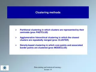
Clustering Methods A Categorization of Major Clustering Methods • Partitioning methods • Hierarchical methods • Density-based methods • Grid-based methods • Model-based methods
Clustering Methods based on Partitioning • Partitioning method: Construct a partition of a database D of n objects into a set of k clusters • Given a k, find a partition of k clusters that optimizes the chosen partitioning criterion • k-means (MacQueen’67): Each cluster is represented by the center of the cluster • k-medoids or PAM method (Partition Around Medoids) (Kaufman & Rousseeuw’87): Each cluster is represented by 1 object in the cluster (~ the middle object or median-like object)
The K-Means Clustering Method Given k, the k-means algorithm is implemented in 4 steps (assumes partitioning criteria is: maximize intra-cluster similarity and minimize inter-cluster similarity. Of course, a heuristic is used. Method isn’t really an optimization) • Partition objects into k nonempty subsets (or pick k initial means). • Compute the mean (center) or centroid of each cluster of the current partition (if one started with k means, then this step is done). centroid ~ point that minimizes the sum of dissimilarities from the mean or the sum of the square errors from the mean. Assign each object to the cluster with the most similar (closest) center. • Go back to Step 2 • Stop when the new set of means doesn’t change (or some other stopping condition?)
k-Means 10 9 8 7 6 5 4 3 2 1 0 0 1 2 3 4 5 6 7 8 9 10 Step 1 Step 2 Step 3 10 9 8 7 6 5 4 3 2 1 0 0 1 2 3 4 5 6 7 8 9 10 Step 4
The K-Means Clustering Method • Strength • Relatively efficient: O(tkn), • n is # objects, • k is # clusters • t is # iterations. Normally, k, t << n. • Weakness • Applicable only when mean is defined (e.g., a vector space) • Need to specify k, the number of clusters, in advance. • It is sensitive to noisy data and outliers since a small number of such data can substantially influence the mean value.
The K-Medoids Clustering Method • Find representative objects, called medoids, (must be an actual object in the cluster, where as the mean seldom is). • PAM (Partitioning Around Medoids, 1987) • starts from an initial set of medoids • iteratively replaces one of the medoids by a non-medoid • if it improves the aggregate similarity measure, retain the swap. Do this over all medoid-nonmedoid pairs • PAM works for small data sets. Does not scale for large data sets • CLARA (Clustering LARge Applications) (Kaufmann,Rousseeuw, 1990) Sub-samples then apply PAM • CLARANS (Clustering Large Applications based on RANdom Search) (Ng & Han, 1994): Randomized the sampling
PAM (Partitioning Around Medoids) (1987) • Use real object to represent the cluster • Select k representative objects arbitrarily • For each pair of non-selected object h and selected object i, calculate the total swapping cost TCi,h • For each pair of i and h, • If TCi,h < 0, i is replaced by h • Then assign each non-selected object to the most similar representative object • repeat steps 2-3 until there is no change
CLARA (Clustering Large Applications) (1990) • CLARA (Kaufmann and Rousseeuw in 1990) • It draws multiple samples of the data set, applies PAM on each sample, and gives the best clustering as the output • Strength: deals with larger data sets than PAM • Weakness: • Efficiency depends on the sample size • A good clustering based on samples will not necessarily represent a good clustering of the whole data set if the sample is biased
CLARANS (“Randomized” CLARA) (1994) • CLARANS (A Clustering Algorithm based on Randomized Search) (Ng and Han’94) • CLARANS draws sample of neighbors dynamically • The clustering process can be presented as searching a graph where every node is a potential solution, that is, a set of k medoids • If the local optimum is found, CLARANS starts with new randomly selected node in search for a new local optimum (Genetic-Algorithm-like) • Finally the best local optimum is chosen after some stopping condition. • It is more efficient and scalable than both PAM and CLARA
Distance-based partitioning has drawbacks • Simple and fast O(N) • The number of clusters, K, has to be arbitrarily chosen before it is known how many clusters is correct. • Produces roundshaped clusters, not arbitrary shapes (Chameleon data set below) • Sensitive to the selection of the initial partition and may converge to a local minimum of the criterion function if the initial partition is not well chosen. Correct result K-means result
Distance-based partitioning (Cont.) • If we start with A, B, and C as the initial centriods around which the three clusters are built, then we end up with the partition {{A}, {B, C}, {D, E, F, G}} shown by ellipses. • Whereas, the correct three-cluster solution is obtained by choosing, for example, A, D, and F as the initial cluster means (rectangular clusters).
A Vertical Data Approach • Partition the data set using rectangle P-trees (a gridding) • These P-trees can be viewed as a grouping (partition) of data • Pruning out outliers by disregard those sparse values Input: total number of objects (N), percentage of outliers (t) Output: Grid P-trees after prune (1) Choose the Grid P-tree with smallest root count (Pgc) (2) outliers:=outliers OR Pgc (3) if (outliers/N<= t) then remove Pgc and repeat (1)(2) • Finding clusters using PAM method; each grid P-tree is an object • Note: when we have a P-tree mask for each cluster, the mean is just the vector sum of the basic Ptrees ANDed with the cluster Ptree, divided by the rootcount of the cluster Ptree
Distance Function X11 … X1f … X1p . . . . . . . . . Xi1 … Xif … Xip . . . . . . . . . Xn1 … Xnf … Xnp 0 d(2,1) 0 d(3,1) d(3,2) 0 . . . . . . . . . . . . . . . d(n,1) d(n,2) … d(n,n-1) 0 • Data Matrix n objects × p variables • Dissimilarity Matrix n objects × n objects
AGNES (Agglomerative Nesting) • Introduced in Kaufmann and Rousseeuw (1990) • Use the Single-Link (distance between two sets is the minimum pairwise distance) method • Merge nodes that are most similarity • Eventually all nodes belong to the same cluster
DIANA (Divisive Analysis) • Introduced in Kaufmann and Rousseeuw (1990) • Inverse order of AGNES (intitially all objects are in one cluster; then it is split according to some criteria (e.g., maximize some aggregate measure of pairwise dissimilarity again) • Eventually each node forms a cluster on its own
Contrasting Clustering Techniques • Partitioning algorithms: Partition a dataset to k clusters, e.g., k=3 • Hierarchical alg:Create hierarchical decomposition of ever-finer partitions. e.g., top down (divisively). bottom up (agglomerative)
Hierarchical Clustering Agglomerative a Step 1 Step 2 Step 3 Step 4 Step 0 a b b a b c d e c c d e d d e e
Hierarchical Clustering (top down) a a b b a b c d e c c d e d d e e Divisive Step 3 Step 2 Step 1 Step 0 Step 4 In either case, one gets a nice dendogram in which any maximal anti-chain (no 2 nodes linked) is a clustering (partition).
Hierarchical Clustering (Cont.) Recall that any maximal anti-chain (maximal set of nodes in which no 2 are chained) is a clustering (a dendogram offers many).
Hierarchical Clustering (Cont.) But the “horizontal” anti-chains are the clusterings resulting from the top down (or bottom up) method(s).
Hierarchical Clustering (Cont.) • Most hierarchical clustering algorithms are variants of the single-link, complete-link or average link. • Of these, single-link and complete link are most popular. • In the single-link method, the distance between two clusters is the minimum of the distances between all pairs of patterns drawn one from each cluster. • In the complete-link algorithm, the distance between two clusters is the maximum of all pairwise distances between pairs of patterns drawn one from each cluster. • In the average-link algorithm, the distance between two clusters is the average of all pairwise distances between pairs of patterns drawn one from each cluster (which is the same as the distance between the means in the vector space case – easier to calculate).
Distance Between Clusters • Single Link: smallest distance between any pair of points from two clusters • Complete Link: largest distance between any pair of points from two clusters
Distance between Clusters (Cont.) • Average Link:average distance between points from two clusters • Centroid: distance between centroids of the two clusters
Single Link vs. Complete Link (Cont.) Single link works but not complete link Completelink works but not single link Completelink works but not single link
Single Link vs. Complete Link (Cont.) 1 1 1 1 1 1 1 1 2 2 2 2 2 2 2 2 1 1 1 1 1 1 Single link works Complete link doesn’t
Single Link vs. Complete Link (Cont.) 2 2 1 1 2 2 1 1 2 2 1 1 2 2 2 2 1 1 2 2 2 2 Single link doesn’t works Complete link does 1-cluster noise 2-cluster
Hierarchical vs. Partitional • Hierarchical algorithms are more versatile than partitional algorithms. • For example, the single-link clustering algorithm works well on data sets containing non-isotropic (non-roundish) clusters including well-separated, chain-like, and concentric clusters, whereas a typical partitional algorithm such as the k-means algorithm works well only on data sets having isotropic clusters. • On the other hand, the time and space complexities of the partitional algorithms are typically lower than those of the hierarchical algorithms.
More on Hierarchical Clustering Methods • Major weakness of agglomerative clustering methods • do not scale well: time complexity of at least O(n2), where n is the number of total objects • can never undo what was done previously (greedy algorithm) • Integration of hierarchical with distance-based clustering • BIRCH (1996): uses Clustering Feature tree (CF-tree) and incrementally adjusts the quality of sub-clusters • CURE (1998): selects well-scattered points from the cluster and then shrinks them towards the center of the cluster by a specified fraction • CHAMELEON (1999): hierarchical clustering using dynamic modeling
Density-Based Clustering Methods • Clustering based on density (local cluster criterion), such as density-connected points • Major features: • Discover clusters of arbitrary shape • Handle noise • One scan • Need density parameters as termination condition • Several interesting studies: • DBSCAN: Ester, et al. (KDD’96) • OPTICS: Ankerst, et al (SIGMOD’99). • DENCLUE: Hinneburg & D. Keim (KDD’98) • CLIQUE: Agrawal, et al. (SIGMOD’98)
Density-Based Clustering: Background p MinPts = 5 = 1 cm q • Two parameters: • : Maximum radius of the neighbourhood • MinPts: Minimum number of points in an -neighbourhood of that point • N(p): {q belongs to D | dist(p,q) } • Directly (density) reachable: A point p is directly density-reachable from a point q wrt. , MinPts if • 1) p belongs to N(q) • 2) q is a core point: |N(q)|MinPts
Density-Based Clustering: Background (II) • Density-reachable: • A point p is density-reachable from a point q (p) wrt , MinPts if there is a chain of points p1, …, pn, p1=q, pn=p such that pi+1 is directly density-reachable from pi • q, q is density-reachable from q. • Density reachability is reflexive and transitive, but not symmetric, since only core objects can be density reachable to each other. • Density-connected • A point p is density-connected to a q wrt , MinPtsif there is a point o such that both, p and q are density-reachable from o wrt ,MinPts. • Density reachability is not symmetric, Density connectivity inherits the reflexivity and transitivity and provides the symmetry. Thus, density connectivity is an equivalence relation and therefore gives a partition (clustering). p p1 q p q o
DBSCAN: Density Based Spatial Clustering of Applications with Noise • Relies on a density-based notion of cluster: A cluster is defined as an equivalence class of density-connected points. • Which gives the transitive property for the density connectivity binary relation and therefore it is an equivalence relation whose components form a partition (clustering) according to the duality. • Discovers clusters of arbitrary shape in spatial databases with noise Outlier Border = 1cm MinPts = 3 Core
DBSCAN: The Algorithm • Arbitrary select a point p • Retrieve all points density-reachable from p wrt ,MinPts. • If p is a core point, a cluster is formed (note: it doesn’t matter which of the core points within a cluster you start at since density reachability is symmetric on core points.) • If p is a border point or an outlier, no points are density-reachable from p and DBSCAN visits the next point of the database. Keep track of such points. If they don’t get “scooped up” by a later core point, then they are outliers. • Continue the process until all of the points have been processed. • What about a simpler version of DBSCAN: • Define core points and core neighborhoods the same way. • Define (undirected graph) edge between two points if they cohabitate a core nbrhd. • The connectivity component partition is the clustering. • Other related method? How does vertical technology help here? Gridding?
OPTICS Ordering Points To Identify Clustering Structure • Ankerst, Breunig, Kriegel, and Sander (SIGMOD’99) • http://portal.acm.org/citation.cfm?id=304187 • Addresses the shortcoming of DBSCAN, namely choosing parameters. • Develops a special order of the database wrt its density-based clustering structure • This cluster-ordering contains info equivalent to the density-based clusterings corresponding to a broad range of parameter settings • Good for both automatic and interactive cluster analysis, including finding intrinsic clustering structure
OPTICS Does this order resemble the Total Variation order?
Reachability-distance undefined ‘ Cluster-order of the objects
DENCLUE: using density functions • DENsity-based CLUstEring by Hinneburg & Keim (KDD’98) • Major features • Solid mathematical foundation • Good for data sets with large amounts of noise • Allows a compact mathematical description of arbitrarily shaped clusters in high-dimensional data sets • Significant faster than existing algorithm (faster than DBSCAN by a factor of up to 45 – claimed by authors ???) • But needs a large number of parameters
Denclue: Technical Essence • Uses grid cells but only keeps information about grid cells that do actually contain data points and manages these cells in a tree-based access structure. • Influence function: describes the impact of a data point within its neighborhood. • F(x,y) measures the influence that y has on x. • A very good influence function is the Gaussian, F(x,y) = e –d2(x,y)/2 • Others include functions similar to the squashing functions used in neural networks. • One can think of the influence function as a measure of the contribution to the density at x made by y. • Overall density of the data space can be calculated as the sum of the influence function of all data points. • Clusters can be determined mathematically by identifying density attractors. • Density attractors are local maximal of the overall density function.
DENCLUE(D,σ,ξc,ξ) • Grid Data Set (use r = σ, the std. dev.) • Find (Highly) Populated Cells (use a threshold=ξc) (shown in blue) • Identify populated cells (+nonempty cells) • Find Density Attractor pts, C*, using hill climbing: • Randomly pick a point, pi. • Compute local density (use r=4σ) • Pick another point, pi+1, close to pi, compute local density at pi+1 • If LocDen(pi) < LocDen(pi+1), climb • Put all points within distance σ/2 of path, pi, pi+1, …C* into a “density attractor cluster called C* • Connect the density attractor clusters, using a threshold, ξ, on the local densities of the attractors. • A. Hinneburg and D. A. Keim. An Efficient Approach to Clustering in Multimedia Databases with Noise. In Proc. 4th Int. Conf. on Knowledge Discovery and Data Mining. AAAI Press, 1998. & KDD 99 Workshop.
BIRCH (1996) • Birch: Balanced Iterative Reducing and Clustering using Hierarchies, by Zhang, Ramakrishnan, Livny (SIGMOD’96 http://portal.acm.org/citation.cfm?id=235968.233324&dl=GUIDE&dl=ACM&idx=235968&part=periodical&WantType=periodical&title=ACM%20SIGMOD%20Record&CFID=16013608&CFTOKEN=14462336 • Incrementally construct a CF (Clustering Feature) tree, a hierarchical data structure for multiphase clustering • Phase 1: scan DB to build an initial in-memory CF tree (a multi-level compression of the data that tries to preserve the inherent clustering structure of the data) • Phase 2: use an arbitrary clustering algorithm to cluster the leaf nodes of the CF-tree • Scales linearly: finds a good clustering with a single scan and improves quality with a few additional scans • Weakness: handles only numeric data, and sensitive to the order of the data record.
BIRCH ABSTRACT Finding useful patterns in large datasets has attracted considerable interest recently, and one of the most widely studied problems in this area is the identification of clusters, or densely populated regions, in a multi-dimensional dataset. Prior work does not adequately address the problem of large datasets and minimization of I/O costs. This paper presents a data clustering method named BIRCH (Balanced Iterative Reducing and Clustering using Hierarchies), and demonstrates that it is especially suitable for very large databases. BIRCH incrementally and dynamically clusters incoming multi-dimensional metric data points to try to produce the best quality clustering with the available resources (i.e., available memory and time constraints). BIRCH can typically find a good clustering with a single scan of the data, and improve the quality further with a few additional scans. BIRCH is also the first clustering algorithm proposed in the database area to handle "noise" (data points that are not part of the underlying pattern) effectively. We evaluate BIRCH's time/space efficiency, data input order sensitivity, and clustering quality through several experiments.
Clustering Feature:CF = (N, LS, SS) N: Number of data points LS: Ni=1=Xi SS: Ni=1=Xi2 Branching factor = max # children Threshold = max diameter of leaf cluster Clustering Feature Vector CF = (5, (16,30),(54,190)) (3,4) (2,6) (4,5) (4,7) (3,8)
Birch Iteratively put points into closest leaf until threshold is exceed, then split leaf. Inodes summarize their subtrees and Inodes get split when threshold is exceeded. Once in-memory CF tree is built, use another method to cluster leaves together. Root CF1 CF2 CF3 CF6 child1 child2 child3 child6 Non-leaf node CF1 CF2 CF3 CF5 child1 child2 child3 child5 Leaf node Leaf node prev CF1 CF2 CF6 next prev CF1 CF2 CF4 next Branching factor, B=6 Threshold, L = 7
CURE (Clustering Using REpresentatives ) • CURE: proposed by Guha, Rastogi & Shim, 1998 • http://portal.acm.org/citation.cfm?id=276312 • Stops the creation of a cluster hierarchy if a level consists of k clusters • Uses multiple representative points to evaluate the distance between clusters • adjusts well to arbitrary shaped clusters (not necessarily distance-based • avoids single-link effect
Drawbacks of Distance-Based Method • Drawbacks of square-error based clustering method • Consider only one point as representative of a cluster • Good only for convex shaped, similar size and density, and if k can be reasonably estimated
Cure: The Algorithm • Very much a hybrid method (involves pieces from many others). • Draw random sample s. • Partition sample to p partitions with size s/p • Partially cluster partitions into s/pq clusters • Eliminate outliers • By random sampling • If a cluster grows too slow, eliminate it. • Cluster partial clusters. • Label data in disk
Cure ABSTRACT Clustering, in data mining, is useful for discovering groups and identifying interesting distributions in the underlying data. Traditional clustering algorithms either favor clusters with spherical shapes and similar sizes, or are very fragile in the presence of outliers. We propose a new clustering algorithm called CURE that is more robust to outliers, and identifies clusters having non-spherical shapes and wide variances in size. CURE achieves this by representing each cluster by a certain fixed number of points that are generated by selecting well scattered points from the cluster and then shrinking them toward the center of the cluster by a specified fraction. Having more than one representative point per cluster allows CURE to adjust well to the geometry of non-spherical shapes and the shrinking helps to dampen the effects of outliers. To handle large databases, CURE employs a combination of random sampling and partitioning. A random sample drawn from the data set is first partitioned and each partition is partially clustered. The partial clusters are then clustered in a second pass to yield the desired clusters. Our experimental results confirm that the quality of clusters produced by CURE is much better than those found by existing algorithms. Furthermore, they demonstrate that random sampling and partitioning enable CURE to not only outperform existing algorithms but also to scale well for large databases without sacrificing clustering quality.