Evolutionary Models for Multiple Sequence Alignment

1. Evolutionary Models for Multiple Sequence Alignment CBB/CS 261 B. Majoros

2. Part IEvolutionary Sequence Models

3. The Utility of Evolutionary Models Evolutionary sequence models make use of the assumption that natural selection operates more strongly on some genomic features than others (i.e., functional versus non-functional DNA elements), resulting in a detectable bias in sequence conservation for the features of interest. More generally, conservation patternsmay differ between levels of DNA organization (i.e., amino acids in coding segments, versus individual nucleotides in conserved noncoding elements). (Siepel et al., 2005)

4. Recall: Multivariate HMMs CCATATAATCCCAGGCTCCGCTTCA AGATATCATCAGATGCTACGTATCT N tracks push ... ACATAATATCCGAGGCTCCGCTTCG single emission from a single state Each state emits N residues, one per track—i.e., a column of a multiple alignment. Thus, each state must have a model for the joint distribution of the tracks (to represent emission probabilities). Q: how might we model dependencies between tracks?

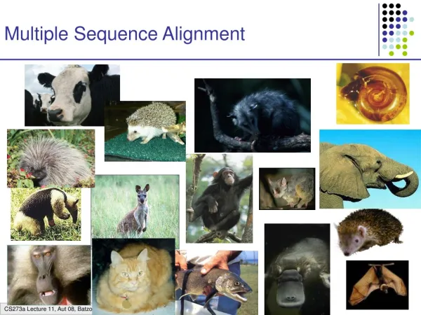
5. Non-independence of Sequences Due to their common ancestry, genomic sequences for related taxa are not independent. We can control for that non-independence by explicitly modeling their dependence structure using a phylogenetic tree: Branch lengths represent evolutionary distance, which conflates the distinct phenomena of elapsed time and substitution rate (as well as selection and drift). We will see later that a phylogenetic tree (or “phylogeny”) can be interpreted as a special type of Bayesian network, in which sequence conservation probabilities are expressed as a function of the branch lengths.

6. PhyloHMMs A PhyloHMM is a discrete multivariate HMM in which each state qi has an associated evolution modeli describing the expected rates and patterns of evolution in the class of features represented by that state. (Siepel et al., 2005)

7. Evaluating the Emission Probability Bayesian network alignment P(G) ...A... ...B... ...C... ...D... G human chimp mouse rat unobservables P(E|G) P(F|G) E F P(C|F) P(A|E) P(D|F) P(B|E) observables A B C D

8. A Recursion for the Emission Likelihood The likelihood can be computed using a recursion known as Felsenstein’s pruning algorithm: =P(descendents of u|u=a). P(c=b|u=a) = probability of observing b in the child, given that we observe a in the parent. We can model this using a matrix of substitution probabilities, parameterized by the evolutionary time t that has passed between the ancestor and descendant taxa: descendant A C G T ancestor A C G T

9. Substitution Matrix vs. Rate Matrix There is an important distinction between a substitution matrix and an instantaneous rate matrix. Q = Instantaneous rate matrix. Gives instantaneous rates of substitutions (not parameterized by time). P(t) = Substitution matrix. Gives the probabilities of substitutions for a specific branch length, t (“time”). Given Q and a set of phylogeny branch lengths {ti}, we can compute a substitution matrix P(ti) for each branch...

10. One Q, Many P(t)’s dolphin whale human kangaroo

11. Continuous-time Markov Chains (CTMCs) Substitution models are typically based on continuous-time Markov chains. The Markov property for CTMCs states that: We can derive an instantaneous rate matrixQ from P(t), where we make use of the fact that P(0)=I. does not depend on t The solution to this differential equation is: eQt (the “matrix exponential”) denotes a Taylor expansion, which we can solve via spectral (eigenvector) decomposition:

12. Desirable Properties of Substitution Matrices Reversibility: ij(πiPij(t)=πjPji(t)) where πi is the equilibrium frequency of base i. (“detailed balance”) Transition/Transversion Discrimination: Using different parameters for transition and transversion rates. Transitions: purinepurine, Transversions: purinepyrimidine pyrimidinepyrimidine

13. Some Common Forms for Q Jukes-Cantor: Kimura: Felsenstein: these assume uniform equilibrium frequencies! Hasegawa, Kishino, Yano: General reversible model:

14. Part IIMultiple Alignment

15. Recall: Pairwise alignment with PHMMs • Emission probabilities assess similarity between aligned residues • Transition probabilities can be used to penalize gaps • Viterbi decoding finds the optimal alignment ε ε D I 1-ε BLOSUM62 δ δ M 1-2δ δ = gap open ε = gap extend

16. Pair HMM  Triple HMM  Quadruple HMM ? for 100bp sequences... pair HMM aligns 2 species triple HMM aligns 3 species #gallons of water in the Pacific ocean quadruple HMM aligns 4 species (Holmes & Bruno, 2001)

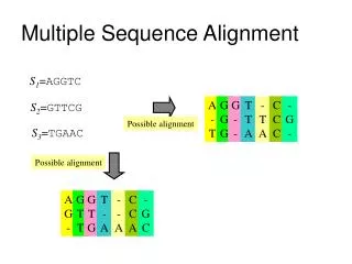
17. Progressive Alignment: One Pair at a Time -AAGTAGCATACG--GGCA-ATT -AACT--CATACG--CCCAGATT T-AGT--CATACGGG--CA-ATC T-AGT--CGTATGGGGGCA-GTT profile-to-profile alignment TAGTCATACGGG--CAATC TAGTCGTATGGGGGCAGTT AAGTAGCATACGGGCA-ATT AACT--CATACGCCCAGATT sequence-to-sequence alignment AACTCATACGCCCAGATT TAGTCATACGGGCAATC AAGTAGCATACGGGCAATT TAGTCGTATGGGGGCAGTT • First, align the leaves of the tree (using a Pair HMM) • Then align ancestral taxa, using either a “consensus” sequence for ancestors, or averaging over all pairs of leaf residues A more principled approach: model the ancestral sequences explicitly, using a probabilistic evolutionary model...

18. Networks of Residues Problem: Align the sequences ABC, DE, FG, and HI. Solution: P Q R S T AB-C- -D-E- --FG- ---HI J K L M N O A B C D E F G H I The multiple alignment problem is precisely the problem of inferring the network of residue homologies—i.e., the evolutionary history of each base.

19. Building the Network D E A B C F G H I ABC DE FG HI

20. Building the Network D E A B C FG- F G -HI H I ABC DE FG HI

21. Building the Network D E A B C unobservables M N O FG- F G -HI F G H I H I observables ABC DE FG HI

22. Building the Network ABC -DE D E A B C M N O FG- F G -HI F G H I H I ABC DE FG HI

23. Building the Network J K L ABC -DE A B C D E D E A B C M N O FG- F G -HI F G H I H I ABC DE FG HI

24. Building the Network J K L A B C D E D E A B C J K L M N O M N O F G F G H I H I ABC DE FG HI

25. Building the Network J K L A B C D E D E A B C J K L M N O M N O F G F G H I H I JK-L- --MNO ABC DE FG HI

26. Building the Network J K L A B C D E D E A B C J K L M N O M N O F G F G H I H I JK-L- --MNO P Q R S T J K L M N O ABC DE FG HI A B C D E F G H I

27. Building the Network J K L A B C D E D E A B C J K L M N O M N O F G F G H I H I P Q R S T AB-C- -D-E- --FG- ---HI J K L M N O ABC DE FG HI A B C D E F G H I

28. Evaluating Emission Probabilities B P(B|K) P(X) J K L X P(K|X) K X P(D|K) D A B C D E P(N|X) M N O N P(G|N) F G H I P(H|N) G H

29. Sampling Alignments = a sequence S = (B,H), a “Branch-HMM” (transducer) B describing the evolutionary process whereby the child evolves from the parent, and the actual indel historyH which is a specific realization of this process (a “draw”) Sampling of alignments proceeds by sampling pairwise “branch alignments” (or “indel histories”) H that live within the yellow squares. An indel history is simply a path through a Pair HMM. Sampling branch alignments is simple: just sample from a PHMM via Forward or Backward:

30. Posterior Alignment Matrix pixel intensity = posterior probability of a match in that cell sequence 2... (posterior probability: conditional on the full input sequences) sequence 1...

31. Banding: Reduce the Search Space

32. Block Rearrangements are a Problem! The simple case: Translocation Inversion Duplication

33. Summary • Optimal MSA computation is intractible in the general case • Progressive alignment is more tractible, but is greedy • Iterative refinement attempts to undo greedy decisions • PairHMM’s provide a principled way to perform pairwise steps • Felsenstein’s algorithm computes likelihoods on phylogenies • Substitution models can use continuous-time Markov chains • Large-scale rearrangements are a problem • Banding can improve alignment speed