Numerical Techniques
Numerical Techniques. Solving a Set of Linear Equations. Example:. + 2 = 1 2 - + 4 = -1 -2 + + 3 = 2. and. where. MATLAB can solve for using matrix left division: x = AB. % Solving a set of linear equations. A = [ 1 2 0 2 -1 4

Numerical Techniques
E N D
Presentation Transcript
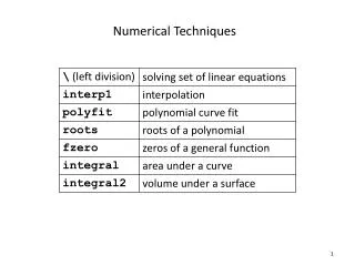
Solving a Set of Linear Equations Example: + 2 = 1 2 - + 4 = -1 -2 + + 3 = 2 and where MATLAB can solve for using matrix left division: x = A\B
% Solving a set of linear equations A = [ 1 2 0 2 -1 4 -2 1 3 ]; B = [ 1 -1 2]'; % t + 2u = 1 % 2t - u + 4v = -1 % -2t + u + 3v = 2 % A*x = B x = A\B; % matrix left division disp(x) disp(['transpose of A*x : ',num2str((A*x)')]) -0.4286 0.7143 0.1429 transpose of A*x : 1 -1 2
Exercise Solve the following set of linear equations: 3- + = -2 - - 2 = 1 2- 2 + 3 = -3
% Linear interpolation x = 0:5; y = [0.15 1.01 1.22 2.54 3.98 4.23]; % data X = linspace(0,5,101); Y = interp1(x,y,X,'linear'); figure(1) plot(x,y,'ko','MarkerFaceColor','k') hold on plot(X,Y,'-r') axis([0 5 0 5])
% Cubic spline interpolation x = 0:5; y = [0.15 1.01 1.22 2.54 3.98 4.23]; % data X = linspace(0,5,101); Y = interp1(x,y,X,'spline'); figure(2) plot(x,y,'ko','MarkerFaceColor','k') hold on plot(X,Y,'-r') axis([0 5 0 5])
Exercise Given the data appearing in the table at the bottom of this slide, do a linear interpolation to find matching y-values for the following set of x-values: 0.5, 1.5, 2.5, 3.5, 4.5
% Curve fitting: 1st-order polynomial x = -3:3; y = [-3.59,-1.71,-0.93,-0.15, 1.27, 1.66, 2.98]; % data coef = polyfit(x,y,1); % 1st-order fit X = linspace(-3,3,61); Y = polyval(coef,X); figure(3) plot(x,y,'ko','MarkerFaceColor','k') hold on plot(X,Y,'-r') axis([-3 3 -4 4])
% Curve fitting: 2nd-order polynomial x = -3:3; y = [9.79, 3.60, 1.35, 0.42, 0.88, 4.11, 8.42]; % data coef = polyfit(x,y,2); % 2nd-order fit X = linspace(-3,3,61); Y = polyval(coef,X); figure(4) plot(x,y,'ko','MarkerFaceColor','k') hold on plot(X,Y,'-r') axis([-3 3 0 10])
Exercise Fit a first-order polynomial (that is, a straight line) to the data in the table at the bottom of this slide. Then prepare a plot with the following: the original data plotted as discrete points and the straight line defined by polyfit. You’ll need to use polyval in order to generate the straight line from the polynomial coefficients.
% Roots of a polynomial coef = [1,-1,-4,4]; % p(x) = x^3 - x^2 - 4x + 4 x = roots(coef); % values of x for which p(x) = 0 disp(x) -2.0000 2.0000 1.0000
Exercise Find the values of that satisfy the following equation:
Function Handle A function handle is a numerical “tag” that identifies a function. It is sometimes more convenient to identify a function by its handle (which is numeric) than by its name (which is a string). A function handle can, for example, be passed as a numerical input argument to another function. An anonymous function is a function that is defined without ever being assigned a name. Every anonymous function will receive a (function) handle, and that is how the function is identified by other parts of the code.
function A = areaCircle(r) • % areaCircle calculates the area of a circle. • % input: r = radius • % output: A = area • A = pi*(r.^2); • end % areaCircle
% Create a function handle • h1 = @areaCircle; % function handle • fprintf('%8.6f\n',h1(1)) • 3.141593
function plotFunction(x,h) • % plotFunction creates a plot, given a function handle. • % Inputs: • % x = abscissa vector • % h = function handle • figure(1) • plot(x,h(x)) • set(gca,'FontSize',20) • xlabel('x’) • ylabel('y’) • title(func2str(h)) • set(findobj(1,'LineWidth',0.5),'LineWidth',2) • saveas(1,func2str(h),'png') • end % plotFunction
% Create an anonymous function having a (function) handle • h2 = @(r) pi*(r.^2); • fprintf('%8.6f\n',h2(1)) • 3.141593
% Find zeros with function fzero NonlinearFunction = @(x) exp(-x) - 0.5; x0 = fzero(NonlinearFunction,[0,1]); fprintf('zero of NonlinearFunction: %6.4f\n',x0) zero of NonlinearFunction: 0.6931
Exercise Find the zero of the function for
% Find area under curve with function integral sinc = @(x) sin(pi*x)./(pi*x); area = integral(sinc,0,4); fprintf('area: %6.4f\n',area) area: 0.4750
Exercise Find the area under the curve for
% Find volume under surface with integral2 Gaussian = @(x,y) exp(-(x.^2 + y.^2)); ymin = @(x) -sqrt(1-x.^2); ymax = @(x) sqrt(1-x.^2); vol = integral2(Gaussian,-1,1,ymin,ymax); fprintf('volume: %6.4f\n',vol) volume: 1.9859
Exercise Find the volume under the surface for (circle of radius 2)