Numerical Integration Techniques
Numerical Integration Techniques. A Brief Introduction By Kai Zhao January, 2011. Objectives. Start Writing your OWN Programs Make Numerical Integration accurate Make Numerical Integration fast CUDA acceleration . The same Objective. Lord, make me accurate and fast.


Numerical Integration Techniques
E N D
Presentation Transcript
Numerical Integration Techniques A Brief Introduction By Kai Zhao January, 2011
Objectives • Start Writing your OWN Programs • Make Numerical Integration accurate • Make Numerical Integration fast • CUDA acceleration
The same Objective Lord, make me accurate and fast. - Mel Gibson, Patriot
Preliminaries • Basic Calculus • Derivatives • Taylor series expansion • Basic Programming Skills • Octave
Numerical Differentiation • Definition of Differentiation • Problem: We do not have an infinitesimal h • Solution: Use a small h as an approximation
Numerical Differentiation Approximation Formula Is it accurate? Forward Difference
Numerical Differentiation Taylor Series expansion uses an infinite sum of terms to represent a function at some point accurately. which implies Error Analysis
Numerical Differentiation Roundoff Error A computer can not store a real number in its memory accurately. Every number is stored with an inaccuracy proportional to itself. Denoted Total Error Usually we consider Truncation Error more. Error Analysis
Numerical Differentiation Backward Difference Definition Truncation Error No Improvement!
Numerical Differentiation Definition Truncation Error More accurate than Forward Difference and Backward Difference Central Difference
Numerical Differentiation Compute the derivative of function At point x=1.15 Example
Use Octave to compare these methods Blue – Error of Forward Difference Green – Error of Backward Difference Red – Error of Central Difference
Numerical Differentiation Multi-dimensional Apply Central Difference for different parameters High-Order Apply Central Difference several times for the same parameter Multi-dimensional & High-Order
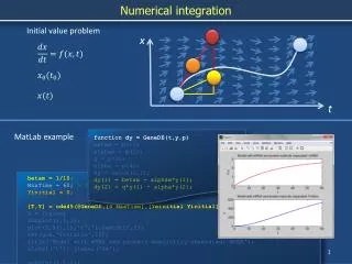
Euler Method The Initial Value Problem Differential Equations Initial Conditions Problem What is the value of y at time t? IVP
Euler Method Consider Forward Difference Which implies Explicit Euler Method
Euler Method Split time t into n slices of equal length Δt The Explicit Euler Method Formula Explicit Euler Method
Euler Method Explicit Euler Method - Algorithm
Euler Method Using Taylor series expansion, we can compute the truncation error at each step We assume that the total truncation error is the sum of truncation error of each step This assumption does not always hold. Explicit Euler Method - Error
Euler Method Consider Backward Difference Which implies Implicit Euler Method
Euler Method Split the time into slices of equal length The above differential equation should be solved to get the value of y(ti+1) Extra computation Sometimes worth because implicit method is more accurate Implicit Euler Method
Euler Method Try to solve IVP What is the value of y when t=0.5? The analytical solution is A Simple Example
Euler Method Using explicit Euler method We choose different dts to compare the accuracy A Simple Example
Euler Method A Simple Example At some given time t, error is proportional to dt.
Euler Method For some equations called Stiff Equations, Euler method requires an extremely small dt to make the result accurate The Explicit Euler Method Formula The choice of Δt matters! Instability
Euler Method Instability Assume k=5 Analytical Solution is Try Explicit Euler Method with different dts
Choose dt=0.002, s.t. Works!
Choose dt=0.25, s.t. Oscillates, but works.
Choose dt=0.5, s.t. Instability!
Euler Method For large dt, explicit Euler Method does not guarantee an accurate result Stiff Equation – Explicit Euler Method
Euler Method Implicit Euler Method Formula Which implies Stiff Equation – Implicit Euler Method
Choose dt=0.5, Oscillation eliminated! Not elegant, but works.
The Three-Variable Model The Differential Equations Single Cell
The Three-Variable Model Simplify the model Single Cell
The Three-Variable Model Using explicit Euler method Select simulation time T Select time slice length dt Number of time slices is nt=T/dt Initialize arrays vv(0, …, nt), v(0, …, nt), w(0, …, nt) to store the values of V, v, w at each time step Single Cell
The Three-Variable Model At each time step Compute p,q from value of vv of last time step Compute Ifi, Iso, Ifi from values of vv, v, w of previous time step Single Cell
The Three-Variable Model At each time step Use explicit Euler method formula to compute new vv, v, and w Single Cell
Heat Diffusion Equations • The Model • The first equation describes the heat conduction • Function u is temperature distribution function • Constant α is called thermal diffusivity • The second equation initial temperature distribution
Heat Diffusion Equation Laplace Operator Δ (Laplacian) Definition: Divergence of the gradient of a function Divergence measures the magnitude of a vector field’s source or sink at some point Gradient is a vector point to the direction of greatest rate of increase, the magnitude of the gradient is the greatest rate Laplace Operator
Heat Diffusion Equation Meaning of the Laplace Operator Meaning of Heat Diffusion Operator At some point, the temperature change over time equals the thermal diffusivity times the magnitude of the greatest temperature change over space Laplace Operator
Heat Diffusion Equation Cartesian coordinates 1D space (a cable) Laplace Operator
Heat Diffusion Equation Compute Laplacian Numerically (1d) Similar to Numerical Differentiation Laplace Operator
Heat Diffusion Equation Boundaries (1d), take x=0 for example Assume the derivative at a boundary is 0 Laplacian at boundaries Laplace Operator
Heat Diffusion Equation • Exercise • Write a program in Octave to solve the following heat diffusion equation on 1d space:
Heat Diffusion Equation • Exercise • Write a program in Octave to solve the following heat diffusion equation on 1d space: • TIPS: • Store the values of u in a 2d array, one dimension is the time, the other is the cable(space) • Use explicit Euler Method • Choose dt, dx carefully to avoid instability • You can use mesh() function to draw the 3d graph
Store u in a two-dimensional array u(i,j) stores value of u at point x=xi, time t=tj. u(i,j) is computed from u(i-1,j-1), u(i,j-1), and u(i+1,j+1).
Heat Diffusion Equation • Explicit Euler Method Formula • Discrete Form
Heat Diffusion Equation • Stability • dt must be small enough to avoid instability