Polar Winds from Satellite Imagers for Numerical Weather Prediction and Climate Applications

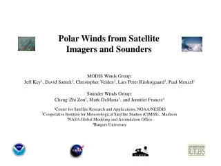
1. Polar Winds from Satellite Imagers for Numerical Weather Prediction and Climate Applications Jeff Key NOAA/National Environmental Satellite, Data, and Information ServiceMadison, Wisconsin USA with lots of help from: Dave Santek, Chris Velden, Matthew Lazzara, William Straka Space Science and Engineering Center, University of WisconsinMadison, Wisconsin USA

2. Satellite-Derived Winds Heritage The polar winds work is building on the long history of geostationary wind retrieval, which began around 1970 when the first geostationary satellites were launched.

3. Targeting • - clouds in the IR window channel 11 mm • - water vapor features in 6.7 mm • Tracking • - cross-correlation technique • - model winds used as first guess • - image triplets (rather than pairs) used for consistency check • Wind height assignment: IR window, CO2-slicing, or H2O-intercept Automated Wind Retrieval Methodology

4. Geostationary Cloud Motion Vectors Five geos provide coverage for winds in the tropics and mid-latitudes. However, the total number of wind vectors drops off steadily beyond a 30 degree view angle, with a sharp drop off beyond 60 degrees. The success rate (#vectors/total possible) drops off beyond 50 degrees.

5. Justification Sparse Observation Network Arctic and Antarctic Rawinsonde Distribution Raob locations are indicated by their WMO station numbers.

6. New Challenges • Reduced temporal sampling compared to GOES • Parallax • Height assignment issues • low-level inversion • isothermal layers • warm, thin clouds over cold surface • low water vapor amounts • Additional spectral channels are available. Are they useful? • Validation

7. Orbits Figures from http://www.rap.ucar.edu/~djohnson/satellite/coverage.html

8. Overpass Frequency The figure at right shows the time of successive overpasses at a given latitude-longitude point on a single day with only the Terra satellite. The figure at the upper right shows the frequency of "looks" by two satellites: Terra and (the future) Aqua. The figure at the lower right shows the temporal sampling with five satellites.

9. One Day of Arctic Orbits, Terra MODIS MODIS band 27 (water vapor at 6.7 mm)

10. Unlike geostationary satellites at lower latitudes, it is not be possible to obtain complete polar coverage at a snapshot in time with one or two polar-orbiters. Instead, winds must be derived for areas that are covered by two or three successive orbits, an example of which is shown here. The whitish area is the overlap between three orbits.

11. Unlike geostationary satellites at lower latitudes, it is not be possible to obtain complete polar coverage at a snapshot in time with one or two polar-orbiters. Instead, winds must be derived for areas that are covered by two or three successive orbits, an example of which is shown here. The whitish area is the overlap between three orbits. Three overlapping Aqua MODIS passes, with WV and IR winds superimposed. The white wind barbs are above 400 hPa, cyan are 400 to 700 hPa, and yellow are below 700 hPa.

12. Spatial and Temporal Resolution Relationships The minimum detectable wind speed as a function of pixel size and time interval, calculated as the pixel size divided by the time interval. For example, with a 4 km pixel and a sampling frequency of 60 minutes, we won't be able to detect speeds less than 1.1 m/s. This could also be viewed as the precision of the measurement; e.g., we will only measure wind speeds in increments of 1.1 m/s at these time and space resolutions. This does not take into account the evolution of tracking features over time, or the increase in spatial variability as pixel size decreases.

13. Infrared Winds Low Level Mid Level High Level 05 March 2001: Daily composite of 11 micron MODIS data over half of the Arctic region. Winds were derived over a period of 12 hours. There are about 4,500 vectors in the image. Vector colors indicate pressure level - yellow: below 700 hPa, cyan: 400-700 hPa, purple: above 400 hPa.

14. Water Vapor Winds Low Level Mid Level High Level 05 March 2001: Daily composite of 6.7 micron MODIS data over half of the Arctic region. Winds were derived over a period of 12 hours. There are about 13,000 vectors in the image. Vector colors indicate pressure level - yellow: below 700 hPa, cyan: 400-700 hPa, purple: above 400 hPa.

15. One Day of Arctic Orbits, Terra MODIS Routine production of MODIS winds began in 2002 with data from the NOAA “bent pipe”. MODIS band 31 (11 mm)

16. Frequency of Water Vapor and IR Winds

17. Height Assignment • Three primary height assignment methods: • CO2 slicing - Problems occur when the clear-cloudy radiance difference is small. Cloud pressures greater than 700 mb (lower in altitude) are generally not retrievable with this method. • H2O intercept - In practice the method is generally not useful for cloud pressures greater than 600-700 mb. • IR Window - This approach assumes the cloud is opaque so that the IR brightness temperature is also the cloud temperature. Ideally, an adjustment for surface emission would be used with thin clouds, which means optical depth must be calculated.

18. Temperature

19. Water Vapor

20. Height Assignment CO2-Slicing Problems occur when the clear-cloudy radiance difference is small. Cloud pressures greater than 700 hPa (lower in altitude) are generally not retrievable with this method. Note difference in horizontal scales.

21. MODIS CO2-Slicing “Failure” Rate in the Polar Regions No CO2 retrieval attemptedbelow 700 hPa No CO2 retrieval found

22. IR Window Currently, this approach assumes the cloud is opaque so that the IR brightness temperature is also the cloud temperature. Find the temperature in the profile to get the height. An adjustment for surface emission should be used with thin clouds, which means optical depth must be calculated. The ISCCP and CASPR methods adjust cloud temperature if the IR optical depth is less than 4.6 (> 1% transmission), which is a larger visible optical depth for water clouds but somewhat smaller for ice clouds.

23. Converting the cloud temperature to a cloud pressure (lookup in the profile), the adjustment in summer will generally increase the cloud altitude. In winter the direction of change may be mixed due to inversions. The point-by-point retrievals, with and without the adjustment for optical depth, are shown above for one summer image. Only clouds with visible optical depths less than 5 are shown. The relative frequency of the pressure differences is shown at left.

24. Note slope differences for low clouds H2O-Intercept Problem: 6.7 m band is insensitive to low clouds. In theory the 7.2 m band, which peaks in the lower troposphere, would be better. In practice the method is generally not useful for cloud pressures greater than 600 mb for 6.7 m and 750 hPa for 7.2 m. 6.7 m 7.2 m

25. Can the 6.7 m band see the surface? (cont.) This is a MODIS image covering part of the Arctic (SE Greenland) on 19 March 2001. Surface features are clearly seen in the IR window band (left), but are also apparent in the water vapor band (right). 11 m 6.7 m

26. There is an official NOAA/NESDIS operational MODIS polar winds product, but there is no official NASA product, e.g., no MODxx. The current products are: Near real-time (2-4 hr delay) MODIS winds for the Arctic and Antarctic, distributed by NESDIS and by CIMSS/UWisconsin. Real-time winds from the McMurdo, Antarctica direct broadcast site. Soon to come: Tromsø DB winds! Historical Arctic and Antarctic AVHRR winds, 1981-2002, for use in reanalysis projects. The MODIS Winds Product

27. Using Winds in Operational Forecast Systems: • European Centre for Medium-Range Weather Forecasts (ECMWF) • NASA Global Modeling and Assimilation Office (GMAO) • Japan Meteorological Agency (JMA) • Canadian Meteorological Centre (CMC) • US Navy, Fleet Numerical Meteorology and Oceanography Center (FNMOC) • UK Met Office • National Centers for Environmental Prediction (NCEP/EMC & JCSDA) • Deutscher Wetterdienst (DWD) • NCAR Antarctic Mesoscale Model (AMPS) MODIS Winds in NWP

28. Thinning demonstration:

29. Thinning demonstration:

30. ECMWF Impacts Pre ops tests in 2002 500 hPa geo potential North Atlantic Europe Positive Impact on Weather Forecasts Demonstrated By ECMWF, NASA GMAO, and others

31. Forecast Busts (GMAO) Southern Hemisphere Extratropics Arctic Blue is forecast with MODIS winds; red is control run

32. Impact of MODIS Winds in the Tropics and on Hurricane Track Forecasts (JCSDA) AVERAGE HURRICANE TRACK ERRORS (NM) FREQUENCY OF SUPERIOR HURRICANE PERFORMANCE (%)* • Percent of cases where the specified run had a more accurate hurricane position than the other run. • Note: These cases are for hurricanes in the subtropics.

33. MODIS winds filling observing system void Being used operationally since Jan 2003

34. ECMWF: Error Propagation to the Midlatitudes This animation illustrates the propagation of analysis errors from the poles to the midlatitudes for one case study. Each frame shows the 500 hPa geopotential height for forecasts from 1 to 5 days in 1 day increments. The solid blue line is the geopotential from the experiment that included MODIS winds; the dashed black line is the control (CTL) experiment without MODIS winds. Solid red lines show positive differences in the geopotential height (MODIS minus CTL), and thick dashed green lines show negative differences. The area of large positive differences near the Beaufort Sea (north of Alaska) moves southward over the 5-day period. The CTL run is forming a deeper trough over central Alaska and then over the Pacific south of Alaska than the MODIS run. The 5-day MODIS forecast verifies better against the subsequent analysis (not shown), so the initial analysis for this MODIS forecast was closer to the “truth” than the CTL (positive impact on forecast). The propagation of differences is therefore also a propagation of analysis errors in the CTL forecast. Better observations over the poles should improve forecasts in the midlatitudes.

35. Error Propagation to the Midlatitudes: Snowfall Accumulated snowfall forecasts (mm water equivalent) over Alaska for 20 March 2001. Inclusion of MODIS winds in the analysis can produce a more accurate forecast. At right is the snowfall from the 5-day Control forecast (no MODIS winds); below left is the snowfall from the 5-day forecast that included the MODIS winds in the analysis; below right is the snowfall from a 12-hr forecast for verification (“truth”).

36. MODIS Polar Winds Real-Time Processing Delays - Frequency of Delays in Wind Retrievals With an average delay of 3-5 hours, MODIS winds do not meet the 3-hr cutoff for regional/limited area data assimilation systems. Possible solution: Generate winds with direct broadcast data, either on- or off-site.

37. X-band Satellite System at McMurdo Station, Antarctica An L/S/X-band ground station was installed at McMurdo station in January 2005. • The system is a SeaSpace design with a 2.4 meter dish, three computing systems with powerful processing capability. • McMurdo station now has the capability to capture and process AQUA and TERRA satellite data. • The system is also one of the first to be able to capture all telemetries available: L-band NOAA, S-band DMSP and X-Band AQUA/TERRA. • The system supports Antarctic flight and field operations.

38. MODIS Polar Winds Real-Time Processing Time - Direct Broadcast MODIS Data at McMurdo Processing times are for the middle image in a 3-orbit triplet. Actually processing time from image acquisition to availability of wind vectors is 100 minutes (1.67 hrs) less than shown. MODIS images are available (image acquisition to level 1b) in 20-30 minutes. Winds processing takes an additional 10-15 minutes.

39. http://stratus.ssec.wisc.edu/db/mcmurdo Current Products at McMurdo(all MODIS):WindsCloud mask*Cloud pressure*Cloud phase*Total precipitable water*Inversion strengthInversion depthIce/snow surface temperatureIce/snow albedoPlanned products:Ice motion (MODIS + AMSR-E)Ice ageCloud optical properties*IMAPP/MODIS Science Team products

40. Examples of McMurdo DB MODIS Products

41. Examples of McMurdo DB MODIS Products

42. Examples of McMurdo DB MODIS Products

43. Examples of McMurdo DB MODIS Products

44. MODIS Direct Broadcast Sites Next Steps: Arctic Direct Broadcast Sites • Station masks for • Fairbanks, Alaska • Tromsø, Norway • Svalbard Svalbard

45. Another Potential Antarctic Site: Troll Troll (Norway)

46. Climate Application: Reanalysis Model Wind Errors: Francis, 2002 (GRL) examined differences between NCEP/NCAR and ECMWF Reanalysis winds and raob winds for raobs that were not assimilated in the reanalysis, from the LeadEx (1992) and CEAREX (1988) experiments. It was found that both reanalyses exhibit large biases in zonal and meridional wind components, being too westerly and too northerly. Winds are too strong by 25-65%.

47. Historical AVHRR Polar Winds Project 1981-2002 Yellow: Below 700 hPa Light Blue: 400-700 hPa Magenta: Above 400 hPa NOAA-14 August 14, 1995 2300 UTC NOAA-11 August 5, 1993 1800 UTC