Download
1 / 40
560 likes | 894 Views
Numerical Weather Prediction. Numerical Weather Prediction. Dynamical Cores Definitions Grid architectures Time stepping (hydrostatic vs. non-hydrostatic models) Physical Parameterizations Basic Concept Planetary Boundary Layer (PBL) Land-surface models Grid-scale Microphysics

E N D
Numerical Weather Prediction M. D. Eastin
Numerical Weather Prediction • Dynamical Cores • Definitions • Grid architectures • Time stepping (hydrostatic vs. non-hydrostatic models) • Physical Parameterizations • Basic Concept • Planetary Boundary Layer (PBL) • Land-surface models • Grid-scale Microphysics • Sub-grid-scale Convection • Data Assimilation • Available observations • Assimilation techniques • Ensemble Forecasting • Basic Concept • Methods • Advantages and limitations M. D. Eastin
Dynamical Core • Grid “Cells” vs. Grid “Points”: • Numerical models must provide a • spatially-continuous representation • of the full atmosphere • “Points” represent small areas with • large area between adjacent points • “Cells” represents large areas with • no area between adjacent cells • Example: Temperature – the single value • reported represents a spatial average • across the total grid cell area • Cloud cover – the single value • reported represents the fraction • of the total grid cell area occupied • by cloud M. D. Eastin
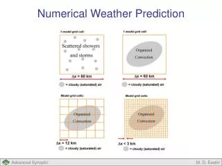
Dynamical Core • Grid “Resolution” vs. Grid “Spacing”: • The effective grid resolution is not the same • as the grid cell spacing • It takes several grid cells to truly resolve the • spatial structureof a meteorological feature • Where is the feature’s maximum? • Where are the feature’s edges? • Model resolution is typically 5 timesthe grid • cell spacing (at a minimum it is 3 times) M. D. Eastin
Dynamical Core • Horizontal Grid Architecture: • Modern models use staggered grids • Mass (or thermodynamic) variables • are computed for the grid cell center • Wind (or kinematic) variables are • computed along grid cell boundaries • Such configuration improves the • model’s computational efficiency • and increases the effective resolution • since the winds only advect mass • across grid cell boundaries • The NAM / WRF model and the • RUC model use this staggered • grid architecture M. D. Eastin
Dynamical Core • Horizontal Grid Architecture: • Some models use spectral coordinates • Represent global atmospheric structure • as the sum of sine and cosine waves • over a range of zonal wavenumbers (n) • Both the GFS model and ECMWF model • are global spectral forecast systems • Advantage: Removes “truncation errors” • that occur when strong gradients are • present between adjacent grid cells • Limitation: Many processes cannot be • represented with spectral techniques • [Precipitation / Vertical advection] • and must still be represented in grid • cell space. • Operational models are really hybrid models – utilizing a variety of numerical techniques to integrate the governing equations Observed SIN n=2 COS n=1 SIN n=1 M. D. Eastin
Dynamical Core • Horizontal Grid Architecture: • Some models use spectral coordinates • Represent atmospheric structure as • the sum of sine and cosine waves over • a wide range of zonal wavenumbers (n) • Example: • If we were to represent a given variable • (temperature) using the first 30 waves • in the zonal direction (n=1–30) then, the • model’s effective grid spacing would be • related to the zonal wavelength (λ) of • the smallest resolved wave (n=30) via • λn=30 = 444 km • The current GFS model analyzes the • first 574 waves (n = 574) for an effective • grid cell spacing of ~23 km Observed SIN n=2 COS n=1 SIN n=1 M. D. Eastin
Dynamical Core • Vertical Grid Architecture: • Some models use sigma coordinates • where: p = pressure at a given level • pT = pressure at the model top • pS = pressure at the surface • σ = 1 at the surface • σ = 0 at the model top • The ECMWF model uses the sigma • coordinate system • Advantage: Model is configured on pressure surfaces (like upper-air observations) • Limitation: Large numerical errors in computing the horizontal pressure gradient • can occur in mountainous regions M. D. Eastin
Dynamical Core • Time Stepping: CFL Condition • In 1928, three mathematicians Courant-Fredrich-Lewy (CFL) determined that numerical • models require a small time step (relative to the grid cell spacing) or numerical instabilities • will occur and the model will generate very large errors (and “crash”) • Condition: where: c = fastest possible wave or wind • Δx = grid cell spacing • Δt = time step between forecasts • Time Stepping: “Advantages” of hydrostatic models • The hydrostatic approximation eliminates small-scale pressure perturbations and • pressure only varies over large (i.e., synoptic) horizontal scales • Recall from your dynamics course that sounds wavesare essentially small-scale pressure • fluctuations that move very quickly (the speed of sound in air is > 300 m/s) • Hydrostatic models have less restrictive CFL conditions c = 100 m/s Δx = 10 km • and thus can complete a full forecast in less time Δt ≤ 100 s • Non-hydrostatic models must account for sounds waves c = 400 m/s Δx = 10 km • with stricter CFL conditions, and thus require more time Δt ≤ 25 s • to complete a full forecast M. D. Eastin
Dynamical Core • Time Stepping: “Advantages” of hydrostatic models • Since hydrostatic models run much faster, long-term prediction (all climate simulations • and many weather forecast models) requirethe hydrostatic approximationin order to • get results in a reasonable amount of “real” time • The “most advanced” modern climate models running on the “fastest” • supercomputers still require 1-2 months to complete 100-year simulations • run in “hydrostatic mode” • As a result – all vertical motions in climate models are diagnosed • Only regional mesoscalemodels are non-hydrostatic • Hydrostatic models: GFS model (global weather/climate) • ECMWF model (global weather/climate) • CCM (global climate) • Non-hydrostatic models: NAM / WRF model • RUC model • MM5 • Hurricane WRF • What does the lackof non-hydrostatic vertical motions imply about ALL climate simulations? M. D. Eastin
Physical Parameterizations • Basic Concept: • Regardless of model type (grid vs. spectral) or model resolution, there are always • physical process that cannot be explicitly resolved by the model. • Any process that occurs on a spatial scale smaller than a grid cell length must be • represented through analytic approximations • Radiation (< 1 m) • Cloud Microphysics (< 1 m) • Planetary Boundary Layer (< 1 km) • Land-surface Processes (< 1 km) • Convection (< 1 km) • Parameterization: The means of expressing unknown or • unresolved quantities in terms of other • existing dependent variables (T, p, u, etc.) • Accounting for unresolved physical • processes without introducing additional • dependent variables • [ Remember: a numerical model consists ] • [ of a “closed set” of N equations with ] • [ N unknowns - or dependent variables ] M. D. Eastin
Physical Parameterizations • Planetary Boundary Layer (PBL): • The atmospheric PBL is a critical component of the “Earth System” since ALLheat, • moisture, and momentum exchange between the atmosphere and the underlying • surface occurs here – particularly in the surface and viscous sub-layers • Then, small-scale 3-D turbulence must transfer the energy from the surface layer • through the mixed layer and into the free atmosphere M. D. Eastin
Physical Parameterizations • Planetary Boundary Layer (PBL): • We have to represent sub-grid-scale 3-D turbulence in terms of grid-scale quantities • without introducing any new predicted (or dependent) variables • Surface-Layer “Closure” Methods: • Bulk Aerodynamic: • Heat Flux • K-theory: • Heat Flux • Monin-Obukov Similarity Theory • see http://glossary.ametsoc.org/wiki/Monin-obukhov_similarity_theory Note:Primes represent the sub-grid-scale [turbulent fluxes] Overbars represent the grid-scale [large-scale means] CH and KH are turbulent transfer coefficients determined through numerous field and lab experiments M. D. Eastin
Physical Parameterizations • Planetary Boundary Layer (PBL): • We have to represent sub-grid-scale 3-D turbulence in terms of grid-scale quantities • without introducing any new predicted (or dependent) variables • Mixed-Layer “Closure” Methods: • Local: Only mix turbulent quantities • up/down to an adjacent model • level through the PBL • Implies that all turbulent mixing • is accomplished by eddies of • of the same small size • Non-local: Can mix turbulent quantities • up/down through all model • levels in the PBL • Implies that turbulent mixing • is accomplished by eddies on • a broad range of scales • Most realistic (and more complicated) M. D. Eastin
Physical Parameterizations • Land-Surface Processes • We have to correctly represent the land surface type, vegetation, and soil properties in • order to properly predict surface layer fluxes, PBL processes, convective initiation, and • precipitation type/amount • Example: Differences in the PBL humidity • due to rapid evapotranspiration • from a corn field and relatively • slow evaporation from a nearby • bare soil field may influence • whether storms develop • Predict: Soil temperature/moisture • Factors: Local albedo • Soil type • Vegetation type • Seasonal vegetation change • Snow cover Noah Land-Surface Model (used in the NAM and GFS models) M. D. Eastin
Physical Parameterizations • Grid-Scale Microphysics: • We have to correctly account for the latent heat release / absorption from water phase • changes of water during cloud and precipitation processes • We must also accurately predict the precipitation type / amount • Predicts: Degree of super-saturation • Latent heat release / absorption • Number concentrations of hydrometeor particles as a function of diameter • [Six types: cloud water, cloud ice, rain, snow, graupel, and hail ] • Fall velocities of each hydrometeor type Lots of small drops Very few large drops M. D. Eastin
Physical Parameterizations • Grid-Scale Microphysics: • We have to correctly account for the latent heat release / absorption from water phase • changes of water during cloud and precipitation processes • We must also accurately predict the precipitation type / amount • Two Types: Bin Method – actually predicts drop counts for each class • Bulk Method – estimates drop counts using analytic formulas M. D. Eastin
Physical Parameterizations • Sub-Grid-Scale Convection: • Often times clouds are smaller than a grid cell – what do we do? • We need to accurately represent the radiation, latent heat, turbulent mixing, precipitation, • and energy transfer associated with such sub-grid-scale clouds. • Convective Parameterizations (CPs): • Required for models run with horizontal grid lengths > 2-3 km • Account for convection in a single grid column • The “triggering” mechanism is unique to each CP scheme • Once “triggered”, all CP schemes adjust the temperature and humidity profile • through the column based of the fractional area covered by convection • Very few CP scheme adjust the momentum fields through the column • [ implies no updrafts or downdrafts – not realistic ] • Numerous CP schemes exist – the most popular ones are: • Betts-Miller-Janjic (BMJ) adjustment scheme • Arakawa-Schubert (AS) mass-flux scheme • Kain-Fritsch (KF) mass-flux scheme M. D. Eastin
Physical Parameterizations • Betts-Miller-Janjic (BMJ) Scheme: • Used in the operationalNAM / WRF regional model • Trigger: Checks grid column for non-zero CAPE extending > 200-mb in depth from the LFC • PBL must have sufficient deep moisture • Requires at most a weak capping inversion M. D. Eastin
Physical Parameterizations • Betts-Miller-Janjic (BMJ) Scheme: • Used in the operational NAM / WRF regional model • Adjustment: If trigger criteria are met, then model adjusts the temperature and humidity • profiles so a net warming (due to latent heat release) and a net drying (due • to moisture removal via precipitation) are achieved through the CAPE layer. No Warming Drying Some Warming Some Drying Warming No Drying M. D. Eastin
Physical Parameterizations • Betts-Miller-Janjic (BMJ) Scheme: • Used in the operationalNAM / WRF regional model • Result: Prolonged triggering of the scheme in a given grid column can be seen • in model forecast soundings as very linear (i.e., unrealistic) profiles • between the LFC and EL • Caused by the lack of downdrafts in the scheme → No cooling in the PBL M. D. Eastin
Physical Parameterizations • Betts-Miller-Janjic (BMJ) Scheme: • Used in the operationalNAM / WRF regional model • Advantages: • Low computational expense due to simplicity • Good performance in moist environments and with afternoon storms • Efficient drying and stabilization of the column • Disadvantages • Neglects cooling due to downdrafts • Inability to trigger convection in dry environments • Difficulty handing convection in capped environments • Does not account well for shallow convection M. D. Eastin
Physical Parameterizations • Arakawa-Schubert (AS) Scheme: • Used in the operationalGFS global model • Trigger: Checks grid column for non-zero CAPE • Checks if column has been destabilizing (has increased CAPE) with time • PBL warming due to advection or surface fluxes • PBL moistening due to advection or surface fluxes • Cold air advection aloft • Radiational cooling aloft • Result: Runs a 1-D cloud model for the cell • Generates an ensemble of clouds • with different depths occupying • some fraction of the grid cell • Reduces the instability in a manner • proportion to its production • Adjusts temperature and moisture • profiles accordingly • Accounts for downdraft cooling, • entrainment / detrainment, and • compensating subsidence M. D. Eastin
Physical Parameterizations • Arakawa-Schubert (AS) Scheme: • Used in the operational GFS global model • Advantages: • Performs well in a variety of environments with realistic sounding adjustments • Represents downdrafts and handles capping inversions • Disadvantages: • Computationally expensive • Performs better with larger grid lengths (> 40 km) in global models M. D. Eastin
Physical Parameterizations • Kain-Fritsch (KF) Scheme: • Not used in any operational models • Common choice in many mesoscale research models • Designed for smaller grid lengths (10-20 km) • Designed for midlatitude continental convection • Trigger: Checks grid column for non-zero CAPE • Checks grid column for sufficient grid-scale vertical motion to lift parcels to LFC • Result: Produces clouds of single depth • (only deep convection) • Accounts for downdraft cooling, • entrainment / detrainment of • both air and hydrometeors at • multiple levels, compensating • subsidence, and storm outflow • Produces realistic adjustments • to the thermodynamic profiles M. D. Eastin
Physical Parameterizations • Kain-Fritsch (KF) Scheme: • Not used in any operational models • Common choice in many mesoscale research models • Designed for smaller grid lengths (10-20 km) • Designed for midlatitude / continental convection • Advantages: • Performs well in mesoscale numerical models • Produces the most realistic cold pools (compared to other CP schemes) • Involves the most realistic entrainment / detrainment processes • Can trigger realistic deep convection in capped environments • Disadvantages: • Large computational expense • Tends to over-moisten the post-convective environment • Does not perform well in other regions (Tropics, over mid-latitude oceans) M. D. Eastin
Physical Parameterizations • Explicit Convection: • When are convective parameterizations schemes no longer needed? • Current estimates suggest that CP is not needed with grid lengths less than 4 km • Why? Many precipitating clouds are greater than 4 km in diameter • All CP schemes were not designed to represent smaller clouds • Nevertheless – great care must be taken to ensure precipitation is accurately represented • (i.e., not “over-predicted”) when no CP scheme is used… No CP Scheme - Explicit Convection BMJ Scheme M. D. Eastin
Physical Parameterizations • Two “Flavors” of Numerical Model Precipitation: • Grid-Scale: Grid cell achieves saturation (or super-saturation) and precipitation • is produced directly via the microphysics scheme • 2. Sub-Grid-Scale: Grid cell does not achieve saturation but does reach the “trigger” criteria • and the convective parameterization schemeproduces precipitation Grid-scale Stratonimbus Contours = Total precipitation Shading = CP precipitation Sub-grid-scale Cumulonimbus M. D. Eastin
Physical Parameterizations • Forecast Sensitivity to CP Choice: • Model forecasts • can change • significantly due • to ONLY choice • of CP scheme!!! • Shown are forecast • fields valid at +30 h • for two numerical • simulations where • the only difference • was the CP scheme SLP and Precipitation 1000-mb θe and winds KF KF BMJ BMJ M. D. Eastin
Data Assimilation • A Not so Simple Requirement for a Good Forecast: • As noted by Bjerknes (1904) - All good forecasts require a sufficiently accurate • knowledge of the state of the atmosphere at the • initial time… • Observations serve a critical role in initializing all weather and climate model simulations – the observations must be accurate • Early Data Assimilation • Generate regularly spaced grids from unevenly distributed observations • Objective analysis (inverse-distance-weighting schemes) • Smoothing (remove small scale “noise”) • Modern Data Assimilation • Combining all available observations to construct the best possible estimate • of the state of the atmosphere • Applied retrospectively to construct “re-analysis” datasets for climate studies • Applied in real-time to initialize weather prediction models • Use very sophisticated analysis techniques – 3DVAR and 4DVAR M. D. Eastin
Data Assimilation • Step-1: Collect Available Observations BIG DATA – TeraBytes collected every hour • In-situ surface observations (ASOS) • In-situ upper air observations (rawinsondes) • In-situ aircraft observations (commercial) • Satellite observations • Imagers (VIS, IR, WV) • IR Sounders (T and RH profiles) • Microwave Sounders (liquid and ice) • Scatterometers (surface winds) • Cloud drift winds • Radar observations (NEXRAD) • Lidar Systems • Unmanned drone aircraft • Neutrally-buoyant balloons M. D. Eastin
Data Assimilation • Step-2: Interpolation of all available data onto an evenly spaced grid • All observations are interpolated onto grids with the same resolution as the model • Data Source Weighting and Influence • Some data types are more reliable than others • (various error magnitudes) • Some data types are more representative than • others (various observed resolutions) • All data types are assigned a unique “weight” • before interpolating and merging with other • data types • Weights are function of both error magnitude • and the spatial distribution of the data source • relative to the other sources • Some data types have more influence on the • the initial conditions than others • These observed fields are NOT BALANCED so… M. D. Eastin
Data Assimilation • Step-3: Creation of a “balanced initial” atmosphere (Analysis) • The weighted / gridded observations are then compared to the “balanced” model field • predicted by the previous forecast cycle but valid at the same data assimilation time • This comparison provides a quantitative • measure of the “distance” between the • observed fields and the fields used to • initialize the model (analysis fields) • This distance is then reduced by applying • “variational techniques” that repeatedly • tweak the analysis fields while maintaining • balance conditions (mass, hydrostatic, • geostrophic, etc.) until an smaller more • acceptable distance is found • This final analysis is then used to initialize • (or start) the numerical simulation • 3DVAR: Observations within a large time window • (±3h) are combined before the analysis • fields are created by variational methods • 4DVAR: Observations are combined into multiple • smaller time windows (< 1h) M. D. Eastin
Ensemble Forecasting • Basic Concept and Purpose: • A prediction based not just a single (deterministic) forecast but on a suite of several • individual forecasts • All non-linear prediction systems suffer from “intrinsic chaos” or “the butterfly effect” • whereby some seemingly miniscule differences in an early model state will amply until • the large-scale forecasts at some later time are completely different • The realistic limit of deterministic prediction is about 2 weeks • Ensemble forecasting is one method used to partially overcome such intrinsic chaos by • quantifying the range (or spectrum) of possible atmospheric states • Sources of Intrinsic Chaos: • Initial Condition Errors: Instrument errors • Errors of representation • Errors in the interpolation process • Small imbalances in the final analyses • Model Errors: Inappropriate physical parameterizations • Inadequate vertical / horizontal resolution • Inadequate representation of boundaries • Unrepresented physical processes ** M. D. Eastin
Ensemble Forecasting • Strategies used to generate an ensemble of forecasts: • The basic operational run of a model is called the control run • An ensemble of additional runs is generated by doing one or all of the following: • Introducing small variations into the initial conditions • Perturbing the model physics (e.g., changing the CP scheme) • Using a suite of different models (WRF, GFS, and ECMWF) • The ensemble meanwill (on average) represent the best forecastwith the smallest error • The range of forecasts from the ensemble can be used to determine forecast confidence M. D. Eastin
Ensemble Forecasting • Advantages: • There are four primary advantages to ensemble prediction beyond what a single • deterministic forecast can provide: • The ensemble mean (based on a simple average or a weighted • average of the individual ensemble members) often exhibits more • skill than do the individual ensemble members • The ensemble provides a quantitative measure of forecast confidence • as a function of lead time and forecast location • A probabilistic forecast is immediately available from the ensemble • The ensemble system provides information regarding the optimal • locations for additional targeted observations which can be used • to improve the forecast (e.g., areas of large standard deviation**) M. D. Eastin
Ensemble Forecasting • Limitation: NOT a “Silver Bullet”: • In some situations the atmosphere can diverge outside the ensemble envelope (range) • Large errors in the initial conditions • Model deficiencies • Unrepresented critical processes M. D. Eastin
Current Operational Forecast Models • GFS Model • Global • Hydrostatic • Spectral (27 km equivalent grid length) • Pressure-sigma (64 vertical levels) • Forecasts out to at least +16 days • 3DVAR (with 6-hr analyses) • 22-member ensemble forecast (MREF) • http://www.emc.ncep.noaa.gov/GFS • ECMWF Model • Global • Hydrostatic • Spectral (25 km equivalent grid length) • Pressure-sigma (91 vertical levels) • Forecasts out to at least +10 days • 4DVAR (with 6-hr analyses) • 51-member ensemble forecast systems • http://www.ecmwf.int/ • NAM / WRF Model • Regional • Non-hydrostatic • Gridded (12 km grid cell length) • Pressure-sigma (35 vertical levels) • Boundary conditions from GFS • Forecasts out to at least +7 days • 3DVAR (with 3-hr analyses) • http://www.emc.ncep.noaa.gov/NAM • RUC / RAP Model • Regional • Hydrostatic • Gridded (13 km grid cell length) • Isentropic-sigma (50 vertical levels) • Boundary conditions from NAM / WRF • Forecasts out to at least +24 hours • 3DVAR (with 1-hr analyses) • http://ruc.noaa.gov/ M. D. Eastin
Model Output Statistics (MOS) • Extracting “Useful” Weather Forecast Information from Numerical Models • Raw numerical forecast fields do not provide • the information desired by the public • Useful MOS is obtained after combining (1) numerical • model output parameters with (2) climatological • information and (3) historical model errors to produce • a new set of statistical forecasts that accounts for • regional and seasonal differences through the use of • multiple linear regression equations • CAUTION: Assumes the model is correct M. D. Eastin
References Barker, D. M., W. Huang, Y. R. Guo and Q. N. Xiao, 2004: A three-dimensional (3DVAR) data assimilation system for use with MM5: Implementation and initial results. Mon. Wea. Rev., 83, 1-10. Bjerknes, V., 1904: The problem of weather forecasting as a problem in mechanics and physics, Meteor. Z., 21, 1-7. Bjerknes, V. 1914: Meteorology as an exact science. Mon. Wea. Rev., 42, 11-14. Kalnay, E, 2003: Atmospheric Modeling, Data Assimilation, and Predictability. Cambridge University Press, 341 pp. Lackmann, G. M., 2011: Winter Storms, Midlatitude Synoptic Meteorology - Dynamics, Analysis, and Forecasting, Amer. Meteor. Soc., Boston, 219-246. Lorenz, E. N., 1965: A study of the predictability of a 28-variable atmospheric model. Tellus, 17, 321-333. Molinari J. and M. Dudek, 1992: Cumulus parameterization in mesoscale numerical models: A critical review. Mon. Wea. Rev., 120, 326-344. Ruth, D. P., B. Glahn, V. Dagostro, and K. Gilbert, 2009: The performance of MOS in the digital age. Weather and Forecasting, 24, 504-519. Strensrud, D. J., H. E. Brooks, J. Du, M. S. Tracton, and E. Rogers, 1999: Using ensembles for short-range forecasting. Mon. Wea. Rev., 127, 433-446. M. D. Eastin