Download
1 / 46
460 likes | 486 Views
Learn about the limitations of uninformed search methods and how informed (or heuristic) search uses problem-specific heuristics, such as best-first, A*, RBFS, and SMA*, to improve efficiency. Discover techniques for generating heuristics and their impact on search complexity. Reading: Chapter 4, Sections 4.1 and 4.2.

E N D
Outline • Limitations of uninformed search methods • Informed (or heuristic) search uses problem-specific heuristics to improve efficiency • Best-first • A* • RBFS • SMA* • Techniques for generating heuristics • Can provide significant speed-ups in practice • e.g., on 8-puzzle • But can still have worst-case exponential time complexity • Reading: • Chapter 4, Sections 4.1 and 4.2
Limitations of uninformed search • 8-puzzle • Avg. solution cost is about 22 steps • branching factor ~ 3 • Exhaustive search to depth 22: • 3.1 x 10¹⁰ states • E.g., d=12, IDS expands 3.6 million states on average [24 puzzle has 1024 states (much worse)]
Recall tree search… This “strategy” is what differentiates different search algorithms
Best-first search • Idea: use an evaluation function f(n)for each node • estimate of "desirability“ • Expand most desirable unexpanded node • Implementation: • Order the nodes in fringe by f(n) (by desirability, lowest f(n) first) • Special cases: • uniform cost search (from last lecture): f(n) = g(n) = path to n • greedy best-first search • A* search • Note: evaluation function is an estimate of node quality => More accurate name for “best first” search would be “seemingly best-first search”
Heuristic function • Heuristic: • Definition: “using rules of thumb to find answers” • Heuristic function h(n) • Estimate of (optimal) cost from n to goal • h(n) = 0 if n is a goal node • Example: straight line distance from n to Bucharest • Note that this is not the true state-space distance • It is an estimate – actual state-space distance can be higher • Provides problem-specific knowledge to the search algorithm
Heuristic functions for 8-puzzle • 8-puzzle • Avg. solution cost is about 22 steps • branching factor ~ 3 • Exhaustive search to depth 22: • 3.1 x 10¹⁰ states. • A good heuristic function can reduce the search process. • Two commonly used heuristics • h1= the number of misplaced tiles • h1(s)=8 • h2= the sum of the distances of the tiles from their goal positions (Manhattan distance). • h2(s)=3+1+2+2+2+3+3+2=18
Greedy best-first search • Special case of best-first search • Uses h(n) = heuristic function as its evaluation function • Expand the node that appears closest to goal
Properties of greedy best-first search • Complete? • Not unless it keeps track of all states visited • Otherwise can get stuck in loops (just like DFS) • Optimal? • No – we just saw a counter-example • Time? • O(bm), can generate all nodes at depth m before finding solution • m = maximum depth of search space • Space? • O(bm) – again, worst case, can generate all nodes at depth m before finding solution
A* Search • Expand node based on estimate of total path cost through node • Evaluation function f(n) = g(n) + h(n) • g(n) = cost so far to reach n • h(n) = estimated cost from n to goal • f(n) = estimated total cost of path through n to goal • Efficiency of search will depend on quality of heuristic h(n)
Admissible heuristics • A heuristic h(n) is admissible if for every node n, h(n) ≤ h*(n), where h*(n) is the true cost to reach the goal state from n. • An admissible heuristic never overestimates the cost to reach the goal, i.e., it is optimistic • Example: hSLD(n) is admissible • never overestimates the actual road distance • Theorem: If h(n) is admissible, A* using TREE-SEARCH is optimal
Optimality of A* (proof) • Suppose some suboptimal goal G2has been generated and is in the fringe. Let n be an unexpanded node in the fringe such that n is on a shortest path to an optimal goal G. • f(G2) = g(G2) since h(G2) = 0 • g(G2) > g(G) since G2 is suboptimal • f(G) = g(G) since h(G) = 0 • f(G2) > f(G) from above
Optimality of A* (proof) • Suppose some suboptimal goal G2has been generated and is in the fringe. Let n be an unexpanded node in the fringe such that n is on a shortest path to an optimal goal G. • f(G2) > f(G) from above • h(n) ≤ h*(n) since h is admissible • g(n) + h(n) ≤ g(n) + h*(n) • f(n) ≤ f(G) Hence f(G2) > f(n), and A* will never select G2 for expansion
Optimality for graphs? • Admissibility is not sufficient for graph search • In graph search, the optimal path to a repeated state could be discarded if it is not the first one generated • Can fix problem by requiring consistency property for h(n) • A heuristic is consistent if for every successor n' of a node n generated by any action a, h(n) ≤ c(n,a,n') + h(n') (aka “monotonic”) • admissible heuristics are generally consistent
A* is optimal with consistent heuristics • If h is consistent, we have f(n') = g(n') + h(n') = g(n) + c(n,a,n') + h(n') ≥ g(n) + h(n) = f(n) i.e., f(n) is non-decreasing along any path. Thus, first goal-state selected for expansion must be optimal • Theorem: • If h(n) is consistent, A* using GRAPH-SEARCH is optimal
Contours of A* Search • A* expands nodes in order of increasing f value • Gradually adds "f-contours" of nodes • Contour i has all nodes with f=fi, where fi < fi+1
Contours of A* Search • With uniform-cost (h(n) = 0, contours will be circular • With good heuristics, contours will be focused around optimal path • A* will expand all nodes with cost f(n) < C*
Properties of A* • Complete? • Yes (unless there are infinitely many nodes with f ≤ f(G) ) • Optimal? • Yes • Also optimally efficient: • No other optimal algorithm will expand fewer nodes, for a given heuristic • Time? • Exponential in worst case • Space? • Exponential in worst case
Comments on A* • A* expands all nodes with f(n) < C* • This can still be exponentially large • Exponential growth will occur unless error in h(n) grows no faster than log(true path cost) • In practice, error is usually proportional to true path cost (not log) • So exponential growth is common
Memory-bounded heuristic search • In practice A* runs out of memory before it runs out of time • How can we solve the memory problem for A* search? • Idea: Try something like depth first search, but let’s not forget everything about the branches we have partially explored.
Recursive Best-First Search (RBFS) • Similar to DFS, but keeps track of the f-value of the best alternative path available from any ancestor of the current node • If current node exceeds f-limit -> backtrack to alternative path • As it backtracks, replace f-value of each node along the path with the best f(n) value of its children • This allows it to return to this subtree, if it turns out to look better than alternatives
Recursive Best First Search: Example • Path until Rumnicu Vilcea is already expanded • Above node; f-limit for every recursive call is shown on top. • Below node: f(n) • The path is followed until Pitesti which has a f-value worse than the f-limit.
RBFS example • Unwind recursion and store best f-value for current best leaf Pitesti result, f [best] RBFS(problem, best, min(f_limit, alternative)) • best is now Fagaras. Call RBFS for new best • best value is now 450
RBFS example • Unwind recursion and store best f-value for current best leaf Fagaras result, f [best] RBFS(problem, best, min(f_limit, alternative)) • best is now Rimnicu Viclea (again). Call RBFS for new best • Subtree is again expanded. • Best alternative subtree is now through Timisoara. • Solution is found since because 447 > 418.
RBFS properties • Like A*, optimal if h(n) is admissible • Time complexity difficult to characterize • Depends on accuracy if h(n) and how often best path changes. • Can end up “switching” back and fortyh • Space complexity is O(bd) • Other extreme to A* - uses too little memory.
(Simplified) Memory-bounded A* (SMA*) • This is like A*, but when memory is full we delete the worst node (largest f-value). • Like RBFS, we remember the best descendant in the branch we delete. • If there is a tie (equal f-values) we delete the oldest nodes first. • simplified-MA* finds the optimal reachable solution given the memory constraint. • Time can still be exponential.
Heuristic functions • 8-puzzle • Avg. solution cost is about 22 steps • branching factor ~ 3 • Exhaustive search to depth 22: • 3.1 x 10¹⁰ states. • A good heuristic function can reduce the search process. • Two commonly used heuristics • h1 = the number of misplaced tiles • h1(s)=8 • h2 = the sum of the distances of the tiles from their goal positions (manhattan distance). • h2(s)=3+1+2+2+2+3+3+2=18
Notion of dominance • If h2(n) ≥ h1(n) for all n (both admissible) then h2dominatesh1 h2is better for search • Typical search costs (average number of nodes expanded) for 8-puzzle problem d=12 IDS = 3,644,035 nodes A*(h1) = 227 nodes A*(h2) = 73 nodes d=24 IDS = too many nodes A*(h1) = 39,135 nodes A*(h2) = 1,641 nodes
Effective branching factor • Effective branching factor b* • Is the branching factor that a uniform tree of depth d would have in order to contain N+1 nodes. • Measure is fairly constant for sufficiently hard problems. • Can thus provide a good guide to the heuristic’s overall usefulness.
Effectiveness of different heuristics • Results averaged over random instances of the 8-puzzle
Inventing heuristics via “relaxed problems” • A problem with fewer restrictions on the actions is called a relaxed problem • The cost of an optimal solution to a relaxed problem is an admissible heuristic for the original problem • If the rules of the 8-puzzle are relaxed so that a tile can move anywhere, then h1(n) gives the shortest solution • If the rules are relaxed so that a tile can move to any adjacent square, then h2(n) gives the shortest solution • Can be a useful way to generate heuristics • E.g., ABSOLVER (Prieditis, 1993) discovered the first useful heuristic for the Rubik’s cube puzzle
More on heuristics • h(n) = max{ h1(n), h2(n),……hk(n) } • Assume all h functions are admissible • Always choose the least optimistic heuristic (most accurate) at each node • Could also learn a convex combination of features • Weighted sum of h(n)’s, where weights sum to 1 • Weights learned via repeated puzzle-solving • Could try to learn a heuristic function based on “features” • E.g., x1(n) = number of misplaced tiles • E.g., x2(n) = number of goal-adjacent-pairs that are currently adjacent • h(n) = w1 x1(n) + w2 x2(n) • Weights could be learned again via repeated puzzle-solving • Try to identify which features are predictive of path cost
Summary • Uninformed search methods have their limits • Informed (or heuristic) search uses problem-specific heuristics to improve efficiency • Best-first • A* • RBFS • SMA* • Techniques for generating heuristics • Can provide significant speed-ups in practice • e.g., on 8-puzzle • But can still have worst-case exponential time complexity • Next lecture: local search techniques • Hill-climbing, genetic algorithms, simulated annealing, etc