Download
1 / 47
480 likes | 499 Views
Explore the advancements, challenges, and future prospects of Least Squares Migration along with case studies and solutions.

E N D
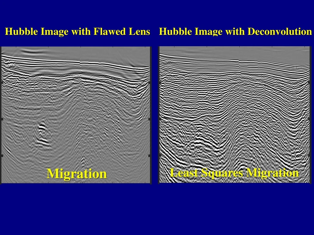
Hubble Image with Flawed Lens Hubble Image with Deconvolution Migration Least Squares Migration
Least Squares Migration: Current and Future Directions Z. Liu, G. Dutta, Y. Huang, W. Dai, X. Wang, & Gerard Schuster KAUST Standard Migration Least Squares Migration
Outline • Least Squares Migration: • Examples of LSM: • Problems with LSM • LSM: PastToday • Road Ahead & Summary
Seismic Inverse Problem m = dm +aLDd m = m +aLDd (k+1) (k) T (k) (k+1) (k) (k) T (k) mig T -1 dm = L d T T T -1 T m= [L L] L d dm= [L L] L d [L L]-1 ~ I Given: d= Lm Find: m(x,y,z) = reflectivity Soln: min || Lm-d||2 + constr. dm LSM Vo fixed (k) mig Vo updated MD migration FWI
Migration Problems 2 Find: min ||Lm - d|| T Soln: m(k+1)= m(k) + a L Dd(k) x-z x-y Problem: mmig=LTd Defocusing Poor resolution Solution: Least squares migration aliasing d Modeling operator m Given: d= Lm = L predicted observed m
Least Squares Migration T m(k+1)= m(k) + a L Dd(k) m= [LTL]-1LT d Source Decon: [w(t) w(t)]-1w(t) w(t) Geom. Spreading: 1 -1 11 r4 r2r2 1/r 1/r Inconsistent events Anti-aliasing: migrate model Aliasing artifacts
Outline • Least Squares Migration: • Examples of LSM: • Problems with LSM • LSM: PastToday • Road Ahead & Summary
Acquisition Footprint Mitigation 5 sail lines 200 receivers/shot 45 shot gathers Standard Migration LSM 0 10 Y (km) 0 10 0 10 X (km) X (km)
RTM vs LSM Reverse Time Migration 0.8 1.2 Z (km) 6.3 9.9 X (km) Plane-Wave LSM 0.8 1.2 Z (km) 6.3 9.9 X (km) Wei Dai (2014)
Outline • Least Squares Migration: • Examples of LSM: • Problems with LSM • LSM: PastToday • Road Ahead & Summary
Problem #1: Erroneous Velocity Problem: High Sensitivity to Inaccurate V(x,y,z) Partial Solutions: a) Statics corrections LSM LSM+Statics LSM CSG1 LSM CSG2 Yunsong Huang (2015) b) Iterative LSM+MVA Sanzong Zhang (2014) RTM+MVA RTM+TraveltimeTomo
Problem #2: Cost Problem: LSM Cost >10x than RTM Solution: Migrate Blended Supergathers
Problem #2: Cost Problem: LSM Cost >10x than RTM Solution: Solution: Approximate [LTL]-1Migration Decon aka Image LSM Deblurring Lm m mmig [LTL] Hu et al. (1998, 2001) Etgen (2002), Aoki (2009) [LTL]-1 Guitton (2002, 2004) Local matching filter
Problem #3: Subsalt Problem: Subsalt Solution: Better v(x,y,z) & Wider Aperture & Fold
Outline • Least Squares Migration: • Examples of LSM: • Problems with LSM • LSM: PastToday • Road Ahead & Summary
Brief History of Least Squares Migration 1983 Linearized Inversion Lailly (1983), Tarantola (1984) 1992 Least Squares Migration Cole+Karrenbach (1992), GTS (1993), Nemeth etal (1996, 1999) Chavent+Plessix (1999), Duquet et al. (2000), Sacchi et al (2006), Tang+Biondi (2009), Zhang et al(2017), Yao+Jacubowicz (2016), Sun etal, (2014-15), Wang etal (2016), Trad (2017), Liu 2018 1998 Migration Deconvolution (aka image domain LSM, deblur) Hu et al. (1998, 2001), Guittonetal (2004), Yu et al. (2006), Aoki +GTS (2009), Cavalcaetal (2012), Fletcher etal (2012), Feng (2018) 2009
Brief History of Least Squares Migration 1983 Linearized Inversion Lailly (1983), Tarantola (1984) 1992 Least Squares Migration Cole+Karrenbach (1992), GTS (1993), Nemeth etal (1996, 1999) Chavent+Plessix (1999), Duquet et al. (2000), Sacchi et al (2006), Tang+Biondi (2009), Zhang et al(2017), Yao+Jacubowicz (2016), Sun etal, (2014-15), Wang etal (2016), Trad (2017), Liu 2018 1998 Migration Deconvolution (aka image domain LSM, deblur) Hu et al. (1998, 2001), Guittonetal (2004), Yu et al. (2006), Aoki +GTS (2009), Cavalcaetal (2012,2018), Fletcher etal (2012-18) 2009 Multisource Least Squares Migration Tang & Biondi (2009), Dai & GTS (2009), Verschuur& Berkhout (2009), Dai (2011, 2012), Zhang et al. (2013), Dai et al. (2012, 2013), and many others (2014)
Brief History of Least Squares Migration 2014 LSM Data-Data Free Surface Multiples Wong et al. (2014), Yang et al. (2015), Tu+Hermmann (2015), Zhang+GTS (2014), Liu et al. (2016), Lu et al. (2018), Whitmore et al. (2018), Chemingui et al. (2018), Zheng et al. (2019) and others M P Multiple->2 bounce pts 2017 LSM Double fold, CDP density 2018
Brief History of Least Squares Migration 2014 LSM Data-Data Free Surface Multiples Wong et al. (2014), Yang et al. (2015), Tu+Hermmann (2015), Zhang+GTS (2014), Liu et al. (2016), Lu et al. (2018), Whitmore et al. (2018), Chemingui et al. (2018), Zheng et al. (2019) and others Viscoacoustic Least Squares Migration Blanch et al. (1998), Plessix (2006), …Dutta et al. (2013,2014), Wang+Chen (2014), Qu et al. (2015), Sun et al. (2015, 2016) Viscoacoustic Migration Deconvolution Cavalca et al. (2015), Fletcher et al. (2016), Chen et al. (2019) 2017 2018
Brief History of Least Squares Migration 2014 LSM Data-Data Free Surface Multiples Wong et al. (2014), Yang et al. (2015), Tu+Hermmann (2015), Zhang+GTS (2014), Liu et al. (2016), Lu et al. (2018), Whitmore et al. (2018), Chemingui et al. (2018), Zheng et al. (2019) and others Viscoacoustic Least Squares Migration Blanch et al. (1998), Plessix (2006), …Dutta et al. (2013,2014), Wang+Chen (2014), Qu et al. (2015), Sun et al. (2015, 2016) Viscoacoustic Migration Deconvolution Cavalca et al. (2015), Fletcher et al. (2016), Chen et al. (2019) Elastic Least Squares Migration Chen+Sachi (2017), Stanton+Saachi (2017), Chen et al. (2017), Duan et al. (2017), Feng+GTS (2017), Dias et al. (2017), Qu et al. (2017), Liu et al. (2018), Yue et al. (2018) and others 2017 Elastic Migration Deconvolution Feng+GTS (2018), 2018
T T Elastic RTM: mp=Lp(dp+ds) & ms=Ls(dp+ds) P-image S-image (1 iteration) (1 iteration) 1 without Deblurring Z (km) 3 (1 iteration) (1 iteration) 1 with Deblurring Z (km) 3 2 18 2 18 X (km) X (km)
Outline • Least Squares Migration: • Examples of LSM: • Problems with LSM • LSM: PastToday • Road Ahead & Summary
Road Ahead Least Squares Migration Goal: Faster & More Accurate Better Velocity: MVA+LSM FWI+LSM Subsalt Migration Decon. +Physics: Viscoelastic+anisotropic Multiples, Full Wave Migration Low Rank ~Hessian m mmig Multisource LSM +Redatuming: Marchenko+LSM Machine Learning +3D Spectral Element Topography Start Sharing Data (Equinor) Large Modeling Codes (Princeton)
Road Ahead 21st Century: [LT L]-1 LT d & Accurate v(x,y,z) 20th Century: LT d
Road Ahead Image Computational Cost vs Year 1024x 1/1024 Quasi-Elastic MD+RTM Elastic FWI 45 Hz MD+RTM 3D chips 32x Acoustic FWI 45 Hz Computer Speed (Hecto-Pflops) $1/32 By 2025 it will be as cheap to run Acoustic LSRTM as it does RTM today Image Computational Cost 1x 2D chips Acoustic RTM 45 Hz $1 1/32x 2005 2015 2025 2035 Calendar Year
GOM Field Data • Marine streamer data. • Contain mainly PP but no PS reflections. • P-image predicts most of the P-wave phases • and amplitudes in the data • S-image mainly compensates for • amplitude-variation-with-offset (AVO) effect CSG 0 Time (s) • Acquisition • 496 shots at an interval of 37.5 m • Cable length = 6 km • 480 receivers at an interval of 12.5 m • Recording time = 10 s 10 Trace Number 480 1
Background Velocity Model Background Vs Model Background Vp Model (m/s) (m/s) 2600 1500 1 2100 1200 Z (km) 3 1600 900 (by scaled Vp) (Bowen Guo, 2016) 2 18 2 X (km) 18 X (km)
Elastic LSRTM Image P-image S-image (40 iterations) (40 iterations) 1 without Deblurring Z (km) 3 (5 iterations) (5 iterations) 1 with Deblurring Z (km) 3 2 18 2 18 X (km) X (km)
Problem #2 with LSM Problem: LSM Cost >10x than RTM Solution: Migrate Blended Supergathers
Standard Migration vs Multisource LSM Romero, Ghiglia, Ober, & Morton, Geophysics, (2000) Given: d1 and d2 Given: d1+ d2 Find: m 1 RTM per shot gather Find: m 1 RTM to migrate many shot gathers Soln: m(k+1) = m(k) + a (L1 + L2)(d1+d2) T T Soln: m=L1 d1 + L2 d2 T T T ] = m(k) + a[L1 d1 + L2 d2 Iteratively encode data so L1Td2 = 0 and L2T d1 = 0 T T + L1 d2 + L2 d1 Benefit: 1/10 reduced cost+memory
Multisource LSM (304 blended shot gathers) SNR=30dB 0 0 b) Standard Migration a) Original Z (km) Z (km) Computational gain 1.48 1.48 9.4 5.4 6.75 X (km) 0 • d) 304 shots/gather • 26 iterations c) Standard Migration with 1/8 subsampled shots Conventional migration: 1 Comp. Gain Shots per supergather 76 152 304 38 6.75 6.75 X (km) X (km) 0 0
Migration Deconvolution (aka Image domain LSM, deblurring, 1-step LSM)
Outline • Least Squares Migration: • Examples of LSM: • Cost & V(x,y,z) Problems with LSM • LSM Current • Summary and Road Ahead
Plane-wave LSRTM of 2D GOM Data • Model size: 16 x 2.5 km. • Source freq: 25 hz • Shots: 515 • Cable: 6km • Receivers: 480 km/s 2.1 0 Z (km) 2.5 1.5 16 0 X (km)
Plane-wave LSRTM of 2D GOM Data • Model size: 16 x 2.5 km. • Source freq: 25 hz • Shots: 515 • Cable: 6km • Receivers: 480 km/s 2.1 0 Z (km) 2.5 1.5 16 0 X (km)
Plane-wave LSRTM of 2D GOM Data • Model size: 16 x 2.5 km. • Source freq: 25 hz • Shots: 515 • Cable: 6km • Receivers: 480 km/s 2.1 0 Z (km) 2.5 1.5 16 0 X (km)
Conventional GOM RTM (cost: 1) (Wei Dai) Plane-wave LSRTM (cost: 12) 0 Z (km) 2.5 Encoded Plane-wave LSRTM (cost: 0.4) Plane-wave RTM (cost: 0.2) 0 Z (km) 2.5 16 0 X (km)
Conventional GOM RTM (cost: 1) (Wei Dai) Plane-wave LSRTM (cost: 12) 0 Z (km) LSM RTM 2.5 Encoded Plane-wave LSRTM (cost: 0.4) Plane-wave RTM (cost: 0.2) 0 Z (km) 2.5 16 0 X (km)
SEG/EAGE Model+MarineData (Yunsong Huang) • sources in total 40m 100 m 16 swaths, 50% overlap 256 sources a swath 6 km 20 m 3.7 km 16 cables 13.4 km
Numerical Results (Yunsong Huang) True reflectivities Conventional migration 6.7 km 3.7 km 256shots/super-gather,16iterations 3.7 km 13.4 km 8 x gain in computational efficiency
Outline • Least Squares Migration: • Examples of LSM: • Cost & V(x,y,z) Problems with LSM • LSM Current • Summary and Road Ahead
True Reflectivity Q Model 0 Z (km) 1.5 0 Z (km) 1.5 Q=20000 Q=20 0 X (km) 2 0 X (km) 2 Acoustic LSRTM Viscoacoustic LSRTM 0 Z (km) 1.5 1.0 -1.0 1.0 -1.0 0 X (km) 2 0 X (km) 2
Outline • Least Squares Migration: • Examples of LSM: • Problems with LSM: Cost and V(x,z) Sensitivity • Multisource LSM: Gulf of Mexico Data • Migration Decon: • Summary and Road Ahead
Outline • Least Squares Migration: • Examples of LSM: • Cost & V(x,y,z) Problems with LSM • LSM Current • Summary and Road Ahead
Least Squares Migration Summary Standard Migration 1. LSM Benefits: Anti-aliasing, better resolution, focusing 2. Cost: O(1)-O(15)> migration …but MLSM+MD can help 3. Sensitivity: Quality LSM = RTM if inaccurate v(x,y,z) 4. Viscoacoustic LSM: Required if Q<25? 5. Broken LSM: Multiples. Quality degrades below 2 km? Collect 4:1 data? 6. Migration Decon: O(1 mig.) vs O(10 mig.) LSM+MD 7. Road Ahead: Iterative MVA+MD+MLSM+Statics
Gulf of Mexico Seismic Survey 4 d Predicted data Observed data 1 Time (s) Lm = d 1 1 0 Lm = d 2 2 Lm = d . . N N . m 6 km
Gulf of Mexico Seismic Survey Predicted data Observed data 2 Goal: Solve overdetermined System of equations for m Lm = d 1 1 Lm = d d 2 2 Lm = d . N N . . m 6 km