Download
1 / 27
270 likes | 448 Views
Tracking Multiple Occluding People by Localizing on Multiple Scene Planes. Saad M. Khan and Mubarak Shah, PAMI , VOL. 31, NO. 3, MARCH 2009, Donguk Seo seodonguk@islab.ulsan.ac.kr 2012.07.21. Introduction(1) .

E N D
Tracking Multiple Occluding People by Localizing on Multiple Scene Planes Saad M. Khan and Mubarak Shah, PAMI, VOL. 31, NO. 3, MARCH 2009, DongukSeo seodonguk@islab.ulsan.ac.kr 2012.07.21
Introduction(1) • Multi view approach to detect and track multiple people in crowed and cluttered scenes • Detection and occlusion resolution • Based on geometrical constructs • The distinction of foreground from background • Using standard background modeling techniques • Planar Homographic occupancy constraint • Using SIFT feature matches and employing the RANSAC algorithm • To track multiple people • Using object scene occupancies
Introduction(2) Examples of cluttered and crowded scenes to test this paper’s approach.
Homographic occupancy constraint(1) (a) The blue ray shows how the pixels that satisfy the homographic occupancy constraint warp correctly to foreground in each view. (b) Foreground pixels that belong to the blue person but are occluding the feet region of the green person satisfy the homographic occupancy constraint (the green ray). This seemingly creates a see-through effect in view 1, where the feet of the occluded person can be detected.
Homographic occupancy constraint(2) • Proposition 1 • The image projections of the scene point given by in any views satisfy both of the following: • for • : the foreground region in view • : the image projection of the scene point • for • : the homography induced by plane from view to view • Proposition 2 (Homographic occupancy constraint) • , for • : the set of all pixels in a reference view • : the homographyinduced by plane from the reference view to view • : the piercing point with respect to lies inside the volume of a foreground object in the scene
Localizing people(1) • : the images of the scene obtained from uncalibrated cameras • : a reference view • : homography of the reference plane between the reference view and any other view • : a pixel in the reference image • : warped to pixel in image • : the observation in images at location
Localizing people(2) • : the event that pixel has a piercing point inside a foreground object • Using Bayes law • : the likelihood of observation belonging to the foreground • Plugging (3) into (2) and back into (1) (1) (2) (3) (4)
Modeling clutter and FOV constraints(1) • Assumed the scene point under examination is inside the FOV of each camera • The concept of an RMS clutter metric of the spatial-intensity properties of the scene • : the variance of pixel values within the th cell • : the number of cells or blocks the picture has been divided into • is defined to be twice the length of the largest target dimension. • They compute the clutter metric for each view at each time instant on the foreground likelihood maps obtained from background modeling. (5)
Modeling clutter and FOV constraints(2) • The first row: images from two of test sequences • The second row: foreground likelihood maps for views in the first row
Modeling clutter and FOV constraints(3) • To assign higher confidence to foreground detected from views with lesser clutter • : a normalizing factor • The overlapping FOV of all cameras • : higher confidence in regions with greater view overlap (6) (7)
Localization at multiple planes • : the homography induced by a reference scene plane between views and • : the homography induced by a plane parallel to • : the vanishing point of the normal direction • : a scalar multiple controlling the distance between the parallel planes • The reference plane homographies between views • Automatically calculated with SIFT feature matches • Using the RANSAC algorithm • Vanishing points for the reference direction • Computed by detecting vertical line segments in the scene and finding their intersection in a RANSAC framework (8)
Localization algorithm (1) • Obtain the foreground likelihood maps . • Model background using a Mixture of Gaussians. • Perform background subtraction to obtain foreground likelihood information • Obtain reference plane homographies and vanishing point of reference direction. • for to • Update reference plane homographies using (8) • Warp foreground likelihood maps to a reference view using homographies of the reference plane. • Warped foreground likelihood maps: • Fuse at each pixel location of the reference view according to (7) to obtain synergy map • end for • Arrange s as a 3D stack in the reference direction
Tracking • Tracking methodology • Based on the concept of spatio-temporal coherency of scene occupancies created by objects • To solve the tracking problem by using a sliding window over multiple frames • Look-ahead technique • : the trajectory of spatio-temporal occupancies by individual • : the spatial localization of the individual in the occupancy likelihood information at time • Localization algorithm for a sliding time window of frames (9)
Graph cuts trajectory segmentation (1) • For a time window of frames • The scene occupancy likelihood information from our localization algorithm: • : 3D grid of object occupancy likelihoods • Arranging s in the dimension • Spatio-temporal occupancy likelihood grid: • To segment into background (nonoccupancies) and object occupancy trajectories with the following criteria: • Grid locations with high occupancy likelihoods have a higher chance of being included in object trajectories. • Object trajectories are spatially and temporally coherent. • Energy function (10)
Graph cuts trajectory segmentation (2) • : the set of all grid locations/nodes in • : the set of grid locations in a neighborhood • : the 4D Euclidean distance between grid locations and • : a normalizing factor • In order to minimize the energy function • Using graph cuts techniques • Undirected graph • The set of vertices • The set of spatio-temporal grid locations augmented by the source and sink vertices: • The set of edges • All neighboring pairs of nodes • The edges between each node and the source and sink • The weights on the edges • -> • The edge contains the source or sink as one of its vertices
Graph cuts trajectory segmentation (3) (a) A sequence of synergy maps at the ground reference plane of nine people (b) The XY cut of the 4D spatio-temporal occupancy tracks
Graph cuts trajectory segmentation (4) (a) Reference view (b) The 3D marginal of the 4D spatiotemporal occupancy tracks at a particular time. Notice the gaps in localizations for each person’s color-coded regions. This is because only 10 planes parallel to the ground in the up (Z) direction were used.
Results and discussions (a) The execution time is linear with both the number of views and number of fusion planes (b) Execution time with varying image resolution. As the resolution increases beyond the cache limit of the GPU, the performance drops
Parking lot data set(2) (a) Total average track error of persons (b) Plot on the top: the detection error (number of false positives + number false negative) The bottom plot: the variation of the people density
Parking lot data set(3) (a) Detection error for utilizing a simple threshold of the occupancy likelihood data compared with trajectory segmentation-based approach. (b) Detection results using a threshold-based approach.
Indoor data set(2) (a) Total average track error over time from the top center of the track bounding box to the manually marked head locations of people. (b) The accumulated detection error (number of false positives + number of false negatives accumulated over time) for different individual planes
Conclusions • To track multiple people in a complex environment • Resolving occlusions and localizing people on multiple scene planes • Using a planar homographic occupancy constraint • Segmentation of individual trajectories of the people • Combining foreground likelihood information from multiple views • Obtaining the global optimum of space-time scene occupancies over a window of frames