Download
1 / 66
660 likes | 828 Views
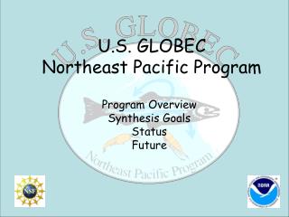
U.S. GLOBEC Northeast Pacific Program. Program Overview Synthesis Goals Status Future. This PPT is used to briefly describe the synthesis research activities of each of the funded NEP synthesis projects (for the November 2006 Pan-Regional Synthesis Meeting).

E N D
U.S. GLOBECNortheast Pacific Program Program Overview Synthesis Goals Status Future
This PPT is used to briefly describe the synthesis research activities of each of the funded NEP synthesis projects (for the November 2006 Pan-Regional Synthesis Meeting). It was compiled by Hal Batchelder and Nick Bond from materials provided by the SIs at various meetings. This material is provided for information purposes only—any use of unpublished material beyond the November PR meeting must be approved by the originating scientist. If you need assistance in identifying whom to contact regarding use of materials here, please email Hal Batchelder at hbatchelder@coas.oregonstate.edu
NE PACIFIC GLOBEC - CORE HYPOTHESES I. Production regimes in the coastal Gulf of Alaska and California Current Systems co-vary, and are coupled through atmospheric and ocean forcing. II. Spatial and temporal variability in mesoscale circulation constitutes the dominant physical forcing on zooplankton biomass, production, distribution, species interactions and retention and loss in coastal regions. III. Ocean survival of salmon is primarily determined by survival of the juveniles in coastal regions, and is affected by interannual and interdecadal changes in physical forcing and by changes in ecosystem food web dynamics.
Hobday and Boehlert (2001) Redrawn from Ware and McFarlane (1999) Coho salmon, Onchorhynchus kisutch, chosen as study species since populations (catch) span and vary inversely in CGOA and CCS, and US GLOBEC and other programs sample in both systems over multiple years.
Spawning Maturing Eggs Ocean Juveniles Salmon Life History Harvest Coastal Shelf Regions Freshwater Other Ocean Areas Adults Diseases/ Parasites Predators Competitors Juveniles Food Supply Salmon Lifecycle Estuary Ocean Physics External Influence Climate Nutrients Courtesy of Ric Brodeur
Pacific Decadal Oscill. Anomaly Patterns SST – colors SLP – contours Windstress - arrows http://www.bom.gov.au/climate/current/soi2.shtml Downwelling Warm phase Cool phase Upwelling ENSO Scale Variability Upwelling Event (Intraseasonal) Variability Pacific Decadal Oscillation Variability
U.S. GLOBEC Northeast Pacific ProgramData Sources • Long-Term Observation Program • Stations • Along-track • Process Cruises • Stations • Along-track • Moorings • Time-series • Drifters • Time-series • Satellite • Time/Space Series • CODAR (CCS only) • Time/Space Series • Modeling • Idealized • Diagnostic Regional • Event driven mesoscale • Retrospective Analysis
GAK 1 GAK 4 GAK 9 Cleare GAK 13 Ocean Carrying Capacity – GLOBEC Trawl Survey Lines August 2001 Seward Line Nutrient Time Series CGOA Sampling Locations
CGOA BPA Trawling (1998-2006) CCS J J F F M M A A M M J J J J A A S S O O N N D D Trawl Survey LTOP Process Trawl Sampling NEP Field Work Timeline Synthesis (2005-2009) 1997-1999 2001 2003 2005 NOPP 2000 COAST 2002 2004 2006
NEP Effort NEP Web Site – http://globec.coas.oregonstate.edu/
Schwing Tynan Casillas Cowles/ Huyer/ Kosro Peterson/ Leising Haidvogel
Top Predators Large-Scale – Mesoscale Thomas Bond Haldorson Salmon Habitat Seasonal/ Interannual Mesoscale Moorings & Transport Euphausiids Climate & Salmon Dagg Copepods Botsford/ Beauchamp Hermann BIOLOGY PHYSICS Core Modeling Batchelder
Large-scale Influences on Mesoscale Structure in the CCS A Synthesis of Climate-forced Variability in Coastal EcosystemsA synthesis of climate-forced variability on mesoscale structure in the CGOA with direct comparisons to the CCS Schwing, Bograd, Mendelssohn, Palacios, Stegmann (SWFSC/ERD); Thomas (U Maine); Strub (OSU)
Project Goals • characterize and compare relationship between basin-scale climate processes and mesoscale physical-ecosystem processes in CCS and CGOA • identify mechanisms by which basin-scale climate variability cascades down to local ecosystem scales • contrast differing CGOA & CCS ecosystem responses to same climate signals • develop indicators representing ecological influences of climate forcing • develop and operate data bases and servers
Synthesis Questions Q1. How did CCS/CGOA mesoscale fields evolve during Field Programs in association with large-scale climate variability? • use correlative methods to characterize mesoscale variability and concurrent basin-scale conditions during Field Programs and extend these comparisons to a longer historical time period where possible. Q2. What are the mechanisms by which large-scale climate forcing cascades to mesoscale variability in CCS/CGOA? • build on correlational linkages between basin and mesoscale patterns of variability and identify possible mechanisms by which local ocean processes respond to climate variability. Q3. How does climate forcing of the CCS and GOA compare? • quantify and compare the relative impact of basin-scale variability on the CGOA and CCS.
West Coast Upwelling Delayed and Weak • Onset of coastal upwelling typically in April-May; July 2005 in northern CC • Stronger upwelling in 2006, but May hiatus • Stronger upwelling late in season, total seasonal upwelling normal but delayed • Weaker upwelling in southern CC in 2005 & 2006 • Delayed upwelling in 2005 & 2006 unusual but not unprecedented • Timing of upwelling and other processes very critical to many species’ reproductive success • Illustrates ecosystem sensitivity to possible future climate extremes
Six “Pipes” Define geostrophic surface velocities in broad channels, using the altimeter SSH along long rows of crossovers, to eliminate the “noise” caused by eddies and Rossby waves. Use tide gauges at the coast to define the SSH, to eliminate any coastal gap. This defines a north and south branch of the N. Pacific Current and broad regions of the California Current and Alaska Current System (Strub, unpublished)
Large changes in the transports in the NPC were seen during the El Nino and especially during 2001-2004, when there was anomalous eastward transports. (Strub, unpublished)
Anomalous chlorophyll in spring 2005: Monthly as a function of latitude – links to wind forcing Monthly Chlorophyll Monthly Ekman Transport climatology climatological variance 2005 2005 (anomalies) Spring negative Large-scale switch from – to + Late-summer positive From Thomas and Brickley (GRL, 2006)
Changing Ocean Conditions in the Northern California Current: Objectives A. Huyer, P. M. Kosro, R. L. Smith, P. A. Wheeler COAS, Oregon State University - relate changing in situphys & chem ocean conditions during 97-03 to primary production; - is interannual variability of phys & chem ocean conditions and primary production similar north and south of Cape Blanco? - do 97-03 seasonal averages & interannual variability of ocean conditions differ from 61-71? - relate present indices of ocean conditions to local in situ measures of the currents, water masses, nutrients, etc., & search for improved indices and measures.
Progress Report: Changing Ocean Conditions in the Northern California Current Ocean Climate Variations Epoch-to-Epoch - average temperatures: winter & summer Year-to-Year - winter & summer T anomalies - water-mass changes (esp. in halocline) - ecosystem response Spatial Differences: NH, CR - midsummer - late summer - spring Specific Events - July 2002 Subduction Event Huyer project
Coho Survival & Climate Indices, 1960-2003 LTOP TENOC Huyer project
Bottom-up Control of Lower-trophic Variability: A Synthesis of Atmospheric, Oceanic and Ecosystem Observations Nick Bond, Cal Mordy, Jeff Napp, Phyllis Stabeno Plan of Attack • Atmospheric Forcing • Local Properties vs. Climate Indices • Along-shore Transport, Cross-shelf Exchange and Mixing • Nutrient Budgets and New Production • Mechanisms Controlling Zooplankton Bond project
Winds Fluor. N+N Salinity Velocity Bond project
Time-Series Measurements “Latitudinal Variation of upwelling, retention, nutrient supply and freshwater effects in the California Current System” M. Kosro, B. Hickey, R. Letelier, S. Ramp A. Mesoscale variability and its alongshore variation, 42-48N, from synthesis of moored (u,v,T,S,chl), HF surface currents, hydrography, and remote sensing. B. Relate physical variability to primary production, zooplankton distributions, and salmon year-class strength. Alongshore variability of upwelling, nutrients, eddies, etc. Interannual variability Relation to higher trophic levels (collaborative with other groups) Kosro project
Temperature and Salinity Near Bottom from WA to Southern OR Kosro project
UNIVERSITY OF WASHINGTON Pink Salmon: Modeling Environmental Effects on Growth & Survival Dave Beauchamp & Alison Cross UW-USGS:Washington Cooperative Fisheries & Wildlife Research Unit Kate Myers, Jan Armstrong, Nancy Davis, Trey Walker UW School of Aquatic and Fisheries Sciences Jamal Moss, NOAA-Auke Bay Lab Ned Cokelet, NOAA-PMEL Lew Haldorson, Jennifer Boldt, Jack Piccolo University of Alaska-Juneau
Scales can be used to estimate growth history S = 3% S = 9% S = 3% S = 8% Ocean Growth and Size-Selective Mortality scale radius ~ fish length circulus spacing ~ growth rate Prince William Sound Pink Salmon -Survivors grow faster than “average” juveniles during first summer Ocean growth -Timing and magnitude of divergent growth between average and surviving Juveniles vary among years -Size-at-age higher for higher survival years Source-Alison Cross, UW High Seas Salmon Group, Jamal Moss, Lew Haldorson
Survival, Growth, Distribution, Diet & Feeding Rate GROWTH: Larger juveniles = Higher survival Critical Period Avg summer Feeding rate: 85-100% of Cmax DISTRIBUTION: Higher survival = Earlier, wider dispersal during Aug-Sep 65-85% Cmax DIET: Diet highly variable among months & Years. Non-Crustaceans Important. Feeding rate higher During High Survival Years— Suggests higher prey availability Jamal Moss, Lew Haldorson, unpub.
Synthesis of Euphausiid Population Dynamics, Production, Retention and Loss under Variable Climatic Conditions William T. Peterson, NMFS, NWFSC, Newport Harold P. Batchelder, Oregon State University Why euphausiids? • Everyone eats them • Numbers and rates highly variable in time and space • Therefore, variations in euphausiid abundance may explain variations in species dependent upon them (e.g., salmon, hake, herring, marine birds) • Euphausiids now incorporated into the Coastal Pelagics Fisheries Management Plan; need to collect data on an going basis, on rates & biomass to properly manage them. • Will develop indices that track interannual variations in euphausiid biomass and productivity Peterson project
Research Activities • Synthesis of target zooplankton abundance and distribution • Seasonal and Interannual variability of nutrients, chlorophyll and ZP • Variability of Euphausiid spawning season • Spatial variations in euphausiid distribution and abundance • Processes that affect abundance and distribution • Stage structure and mortality rates • Egg production • Development time and molting rates • Growth and production • Physical-biological modeling • Population dynamics using IBM’s • Cross-shelf zonation, retention and loss • Future Expansion -- PIRE: The Year of the Euphausiid—Comparative Life History of North Pacific Krill in Shelf and Slope Waters Around the Pacific Rim (proposed, incl. Aust., Kor, Japan, China, Canada, Mexico) Peterson project
Effects of climate variability on Calanus dormancy patterns and population dynamics within the California Current Andrew W. Leising NOAA-SWFSC-ERD 1352 Lighthouse Ave. Pacific Grove, CA 93950 Andrew.leising@noaa.gov Jeffrey Runge, and Catherine Johnson University of New Hampshire Ocean Process Analysis Laboratory Morse Hall 39 College Road Durham, NH 03824 With a lot of help from: Bill Peterson, NOAA; Dave Mackas, IOS; Bruce Frost, UW Leising project
Project Goals: • Determine the most likely factors (biological and physical) that control the dormancy response of Calanus pacificus and Calanus marshallae • These two copepod species often dominate the biomass of macrozooplankton, and are warm/cold indicators • Surprisingly, dormancy triggers remain unknown • Use this information to more accurately model the population response and sensitivity of these species to climate change • Produce a coastwide index of relative population abundance and production of these two species Leising project
Appearance/Dormancy Timing in Relation to Upwelling Increasing Upwelling Decreasing Upwelling C. marshallae almost always wakes up from dormancy during periods of increasing upwelling, and enters dormancy during periods of decreasing upwelling Leising project
Habitat effects on feeding, condition, growth and survival of juvenile pink salmon in the northern Gulf of Alaska P.I.s: Lew Haldorson and Milo Adkison School of Fisheries and Ocean Sciences University of Alaska Fairbanks This work directly addresses NE PACIFIC GLOBEC - CORE HYPOTHESES III. Ocean survival of salmon is primarily determined by survival of the juveniles in coastal regions, and is affected by interannual and interdecadal changes in physical forcing and by changes in ecosystem food web dynamics. Haldorson project
Synthesis Research: I. Compile a comprehensive data set on pink salmon - 4 projects A. LTOP and Process Studies - U. of Alaska B. Ocean Carrying Capacity (OCC) - NFMS, Auke Bay Lab. C. PWS Juvenile Pink Salmon Monitoring - ADF&G, Cordova D. SE Alaska Monitoring Project - NMFS, Auke Bay Lab. II. Examine salmon response variable by year, season, habitat A. Short term - Feeding Intensity (SCI) B. Medium term - Condition (L/W residuals, energy content) C. Long term - Growth (Hatchery fish, exponential, bioenergetic) D. Examine response variable in upper size-based quantiles III. Identify characteristics of habitats associated with positive or negative performance of salmon response variables. A. Temperature B. Stratification C. Zooplankton 1. Direct sampling - process, LTOP, OCC 2. Salmon diets Haldorson project
Juvenile Salmon Habitat Utilization in the Northern California Current – Synthesis and Prediction PI’s – Casillas, Batchelder, Peterson, Brodeur, Jacobson AI’s – Wainwright, Rau, Pearcy, Fisher, Teel, Beckman Principle Hypotheses/Objectives • Habitat for juvenile salmon can be characterized by suite of physical and biological variables (e.g. temperature, salinity, stratification, prey and predator distribution & abundance, etc) • Fine-scale habitat characteristics can be related to meso- to regional-scale ocean features that can be used to construct a ‘salmon ocean habitat index’ to provide near-term prediction of salmon success Casillas project
Example: Logistic Regression Analysis on Presence/Absence; Only statistically significant coefficients shown. Presence/Absence and environmental data from June 1998-2004 cruises used to specify model; Data from June 2005 held in reserve for testing. Bi, Ruppel, and Peterson, Submitted. • Subyearling Chinook:Absence accuracy: 100% Presence accuracy: 17% Overall: 87% • Yearling Chinook: Absence accuracy: 80% Presence accuracy: 75% Overall: 79% • Subadult Chinook:Absence accuracy: 79% Presence accuracy: N/A* Overall: 79% • Yearling cohoAbsence accuracy: 4% Presence accuracy: 100% Overall: 33%** • Subadult cohoAbsence accuracy: 88% Presence accuracy: 100% Overall: 89% Casillas project
What are we doing for management? • Our approach: continue long-term time series. THIS IS CRITICAL! • Need indices based on biological variables, measured on cruises, at the same times-places as the stocks being managed • Developed indices that (so far) predict returns of coho salmon one year in advance; they work because survival is set during the first summer at sea. Supported chiefly by the FATE program (Fisheries and the Environment). • Northern copepod index • Spring Transition Index • Logerwell • Peterson (biological spring transition) • Salmon catches on our Bonneville-funded juvenile salmonid surveys • Coho catches in September predict returns following year • Spring Chinook catches in June predict returns 2-3 years later • Will develop indices based on euphausiids—using easily measured variables (= egg abundances, ratio of eggs/larvae; adult abundances). Casillas project
Casillas project http://www.nwfsc.noaa.gov/research/divisions/fed/climatechange.cfm
Environmental influences on growth and survival of Southeast Alaska coho salmon in contrast with other Northeast Pacific regions Milo Adkison, U.Alaska, Juneau Hal Batchelder, Oregon State U. Nick Bond, NOAA, U.W. Loo Botsford, U.C., Davis Alan Hastings, U.C., Davis Alex Wertheimer, N.M.F.S. Auke Bay Unfunded Collaborator: Marc Trudel (DFO-Canada) Focus on coho salmon, Oncorhynchus kisutch, which does covary out of phase, in CGOA and CCS. Compare on regional (100s of km) to basin scales. Botsford project
Hypotheses H1. Alaska coho salmon survival depends positively on conditions favoring biological productivity.[RETRO, CWT, LOCIND] H2. Alaska coho salmon survival depends on variability in mortality rate due to varying predator buffering by other salmon species.[RETRO, CWT] H3. Survival of coho salmon is determined by availability and spatial arrangement of high quality habitat during early ocean life. [FIELD, IBM] H4. A single model of early growth and survival can explain coho salmon population response to the environment throughout the NEP from the CCS through the CGOA. [CWT, RETRO] Project Components FIELD – coho occurrence, abundance, growth vs. physical/biological IBM – Growth/survival in space/time; including movement/habitat selection RETRO – Expand Auke Creek analysis spatially to examine predator/competitor effects LOCIND – Develop indices of local physical state, e.g., wind stress curl, MLD CWT – Reanalysis of CWT data; fit CGOA and CCS CWT to early life history model with variable grwoth, survival on regional scale Botsford project
NEP U.S. GLOBEC Nested Model Domains Coho Salmon Region Botsford project
How well do the ROMS NEP physics match our perception and data from the real NEP ocean? • Compare SSH from the model with altimetry • Large scale climatology • Seasonality • Compare SST • Compare Subsurface Temperatures • California Undercurrent Strength/Posn/Variability • Interannual Variability in Strength of the Alaskan Gyre Circulation and Bifurcation of the North Pacific Current (particle tracking) Botsford project
Climatological Dynamic Height from Strub and James (2002) 1958-2004 Climatologial SSH from Model Batchelder unpub.
-PDO 1961-75 +PDO 1978-96 From Schwing et al. (2002) The 1976-77 Regime Shift SST Patterns Note: Left panel is May only; Right is Annual Batchelder unpub.
1997 2000 7-8 July 2000 1998 Well defined core of CUC in 1997, 1998, 2000; close to slope 1999 2002 9-11 July 2002 Weaker, more diffuse CUC in 1999 & 2002; not adjacent to slope Northward Velocity – Newport Line - July Batchelder unpub.