k-Coloring
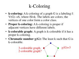
k-Coloring. k-coloring: A k-coloring of a graph G is a labeling f: V(G) S, where |S|=k. The labels are colors; the vertices of one color form a color class. Proper k-coloring: A k-coloring is proper if adjacent vertices have different labels.

k-Coloring
E N D
Presentation Transcript
k-Coloring • k-coloring: A k-coloring of a graph G is a labeling f: V(G)S, where |S|=k. The labels are colors; the vertices of one color form a color class. • Proper k-coloring: A k-coloring is proper if adjacent vertices have different labels. • k-colorable graph: A graph is k-colorable if it has a proper k-coloring. • Chromatic number (G): The least k such that G is k-colorable.
Example 5.1.3 • Petersen Graph: The Petersen graph is the simple graph whose vertices are the 2-element subsets of a 5-element set and whose edges are the pairs of disjoint 2-element subsets. • A graph is 2-colorable if and only if it is bipartite. C5 and Petersen graph have chromatic number at least 3.
k-chromatic graph • k-chromatic graph: A graph G is k-chromatic if (G)=k. A proper k-coloring of a k-chromatic graph is an optimal coloring. • k-critical graph: If (H)< (G)=k for every proper subgraph H of G, then G is k-critical. • Clique Number: The clique number of a graph G, written (G), is the maximum size of clique in G.
Proposition 5.1.7 • For any graph G,(G)>=(G) and (G)<=n(G)/(G). Proof. 1. Vertices of a clique requires distinct colors. (G)>=(G). 2. Each color class is an independent set. (G)<=n(G)/(G).
Example 5.1.8 of (G)>(G) 1. For r>=2, let G=C2r+1Ks. 2. C2r+1 has no triangle (G)=s+2. 3. C2r+1 needs at least three colors, say a, b, and c. 4. Ks needs s colors which must differ from colors a, b, and c. (G)>=s+3.
Greedy Coloring • The greedy algorithm relative to a vertex ordering v1, v2, …, vn of V(G) is obtained by coloring vertices in the order v1, v2, …, vn, assigning to vi the smallest-indexed color not already used on its lower-indexed neighbors.
Proposition 5.1.13 (G)<=(G)+1. Proof. 1. In a vertex ordering, each vertex has at most (G) earlier neighbors. Greedy coloring cannot be forced to use more than (G)+1 colors.
Brook’s Theorem • If G is a connected graph other than a complete graph or an odd cycle, then (G)<=(G). Proof. 1. Let k= (G). 2. Since G is a complete graph when k<=1, and G iss an odd cycle or is bipartite when k=2, in which case the bound holds, we assume that k>=3. 3. The theorem holds if we can order the vertices such that each has at most k-1 lower-indexed neighbors.
Brook’s Theorem (2/6) 4. Case 1: G is not k-regular. Let vn be the vertex of degree less than k. 5. Grow a spanning tree of G from vn, assigning indices in decreasing order as we reach vertices. 6. Each vertex other than vn in the resulting ordering has v1, v2, …, vn has a higher-indexed neighbor along the path to vn in the tree. Each vertex has at most k-1 lower-indexed neighbors.
Brook’s Theorem (3/6) 4. Case 2: G is k-regular. 5. Case 2-1: G has a cut-vertex x. 6. Let G’ be a subgraph consisting of a component of G-x together with its edges to x. 7. The degree of x in G’ is less than k. The method in case 1 provides a proper k-coloring of G’. 8. By permuting the names of colors in the subgraphs resulting in this way from components of G-x, we can make the colorings agree on x to complete a proper k-coloring of G.
Brook’s Theorem (4/6) 9. Case 2-2: G is 2-connected. 10. Suppose that some vertex vn has neighbors v1, v2 such that (v1, v2)E(G) and G-{v1, v2} is connected. 11. Index the vertices of a spanning tree of G-{v1, v2} using 3, 4, …, n such that labels increase along paths to the root vn. 12. Each of v1, v2, …, vn has at most k-1 lower indexed neighbors. 13. v1 and v2 receives the same color. At most k-1 colors are used on neighbors of vn.
Brook’s Theorem (5/6) 14. It suffices to show that every 2-connected k-regular graph with k>=3 has such a triple v1, v2, vn in 10. 15. Choose a vertex x. 16. Case 2-2-1: (G-x)>=2. 17. Let v1 be x and let v2 be a vertex with distance 2 from x. 18. Let vn be a common neighbor of v1 and v2. 19 v1, v2, vn be the desired triple. 20. Case 2-2-2: (G-x)=1.
Brook’s Theorem (6/6) 21. Let vn=x. Then, x has a neighbor in every leaf block of G-x. Otherwise, G is not 2-connected. 22. G-x is not a single block. At least two leaf blocks in G-x. 23. Clearly, neighbors v1 and v2 of x are not adjacent. 24. G-{v1, v2, x} is connected since blocks have no cut-vertices. 25. k>=3. vertex x has a neighbor other than v1 and v2 G-{v1, v2} is connected.
Block-cutpoint graph • Block-cutpoint graph: The block-cutpoint graph of a graph G is a bipartite graph H in which one partite set consists of the cut-vertices of G, and the other has a vertex bi for each block Bi of G. vbi as an edge of H if and only if v Bi.
Leaf Block • Leaf Block: A block that contains exactly one cut-vertex of G. • When G is connected, its block-cutpoint graph is a tree (Exercise 34 of Sec. 4.1) whose leaves are blocks of G. A single block has at least two leaf blocks.