Download
1 / 50
500 likes | 722 Views
HOPF BIFURCATION IN A SYNAPTICALLY COUPLED FHN NEURON MODEL WITH TWO DELAYS. Liping Zhang College of Science, Nanjing University of Aeronautics and Astronautics 2010/07/30. 什么是生物数学?. 生物数学是生物学与数学之间的边缘学科,用数学方法研究和解决生物学问题,也对与生物学有关的数学方法进行理论研究。

E N D
HOPF BIFURCATION IN A SYNAPTICALLY COUPLED FHN NEURON MODEL WITH TWO DELAYS Liping Zhang College of Science, Nanjing University of Aeronautics and Astronautics 2010/07/30
什么是生物数学? • 生物数学是生物学与数学之间的边缘学科,用数学方法研究和解决生物学问题,也对与生物学有关的数学方法进行理论研究。 • 对于今天的生物学者,数学的价值更应该体现在建立在数量化基础上的"模型化"。通过数学模型的构建,可以将看上去杂乱无章的实验数据整理成有序可循的数学问题,将问题的本质抽象出来。
两个最近的事例 • SARS • 在对SARS的研究中,生物数学就发挥了作用。2003年春SARS暴发时,在有效的疫苗和抗病毒药物研制出来之前,科学家最关心的是SARS流行的特征。两个国际合作的研究小组使用了"SEIR"数学模型,对SARS的传播趋势进行分析和预测,给有关部门提供了参考意见。
Avian Influenza Bird flu • Avian influenza is a disease of birds caused by influenza viruses closely related to human influenza viruses. • Transmission to humans in close contact with poultry or other birds occurs rarely and only with some strains of avian influenza. The potential for transformation of avian influenza into a form that both causes severe disease in humans and spreads easily from person to person is a great concern for world health. • Avian Influenza Bird flu
生物数学几个领域的基本介绍 • 种群动力学: 种群的相互作用 生物资源管理和综合害虫控制 • 流行病动力学 • 药物动力学 • 生物数学中的斑图 • 生物信息学
生物数学已有一百年多年的历史: • •1798年Malthus人口增长模型 • •1908年遗传学的Hardy-Weinbe“平衡原理” • •1925年Volterra捕食与被捕食模型 • •1927年KM传染病模型 • •1973年许多著名的生物学杂志相继创刊 • •现如今“生物信息学”的诞生是 • 生物数学发展的里程碑
时滞 • 时滞对生物种群的影响一直是生物学家关心的问题,时滞经常出现在生物的活动中。例如我们日常生活中遇到的视觉和听觉的时滞现象、动物血液再生原理,森林再生原理等。 • 考虑到种群密度变化对于增长率的影响都不是瞬间发生的,而是与过去的生活状态有关, 即有时间滞后的,还有动物消化食物也需要一定的时间。在生物数学模型中如果引入时滞,相应的动力系统就变成了带时滞的非线性动力系统。
目前,对于非线性时滞动力系统尚没有针对性特别强的研究方法,讨论非线性常微分方程的方法,大多可以 经过改造用于非线性时滞微分方程的研究。例如研究生物动力系统平衡点存在唯一性方法有:不动点定理、M-矩阵和重合度理论等;平衡点局部稳定性分析最基本的方法仍是考察特征方程根的变化,例如无害时滞不改变系统正平衡位置的渐近稳定性,所以利用时滞为零时系统的渐近性去研究时滞不为零时系统正平衡位置的局部稳定性,即用线性近似法研究研究平衡点的局部稳定性问题。对小时滞模型用平均法,对常数时滞以及连续时滞模型的全局稳定性主要用Lyapunov方法。研究分岔现象的常见方法有:中心流形法、规范形理论、Lyapunov-Schmidt方法、摄动法和多尺度法等。
1.assumptions • The basic model makes the following assumptions: • (H) • The model is given by the following system:
Fan D, Hong L. Hopf bifurcation analysis in a synaptically coupled FHN neuron model with delays. • Commun Nonlinear Sci Numer Simulat (2009), doi:10.1016/j.cnsns.2009.07.025
2.Stability for FHN neuron model with one delay • Obviously, E (0,0,0,0) is an equilibrium of system (1), linearizing it gives
The characteristic equation associated with system (2) is given by , , Where
For and , Eq.(3) becomes (4) By Routh-Hurwitz criterion we know that if (H) is satisfied then all roots of Eq.(3) have negative real parts.
3.Bifurcation for FHN neuron model with one delay • Obviously, iv(v>0) is a root of Eq.(4) if and only if (5) Separating the real and imaginary parts gives ( (6)
Taking square on the both sides of the equations of (6) and summing them up ,and let y=v2 , which leads to: • where (7)
Denote (8) Then we have (9) Set (10)
Let , then (10) becomes (11) where , Define (12)
Without loss of generality, we assume that Eq.(7) has four positive roots, denoted by ,, and , respectively. Then Eq.(6) has the four positive roots we have (13)
(14) Then Where k=1,2,3,4; is a pair of purely imaginary roots Similar to the proves of [8] we know that of Eq.(4) with Eq.(7) has more than one positive roots. Then the stability switch may exist. Summarizing the above discussions we can ensure the stability interval.
Theorem 3.1 Suppose that (H) is satisfied and • If the conditions (a) (b), △ , and (c) ,△ , and there exists a such that and are not satisfied, then the zero solutions of system ( 1) is asymptotically stable for all . • If one of the conditions (a),(b) and (c) of (1) is satisfied, then the zero solution of system (1) is asymptotically stable when • If one of the conditions (a),(b) and (c) of (1) is satisfied,and , then the system (1) undergos a Hopf bifurcation at (0,0,0,0) when
4.Stability and Hopf bifurcation for FHN neuron model with two delay • Now let be a root of Eq.(2) Then we get (16) Where
Taking square on the both sides of the equations of (14), we get (15) (15)
If Eq.(15) has positive root, without loss of generality , we assume Eq.(15) has N positive roots, denoted by 。Notice Eq.(12)we get (16)
Define • .Let be the root of Eq.(4) • Satisfying • . By computation, we get
Where • Summarizing the discussions above, we have the following conclusions.
Theorem 4.1 Suppose that (H), hold and Eq.(14) has positive roots. and have the same meaning as last definition. We get • (1) All root of Eq.(4) have negative real parts for • and the equilibrium of system (2) is asymptotically stable for . • (2) If hold , then system (2) undergos a Hopf bifurcation at the equilibrium E, when .
5.Stability and direction of the Hopf bifurcation • In the previous section, we obtained conditions for Hopf bifurcation to occur when • . In this section we study the direction of the Hopf bifurcation and the stability • of the bifurcation periodic solutions when , using techniques from normal form and center manifold theory.
Letting • We assume and dropping the bars for simplification (17)
Where and (18) Where
From the discussion in Section 2, we know that system (10) undergos a Hopf bifurcation at (0,0,0) when , and the associated characteristic equation of system (10) with • has a pair of simple imaginary roots • .
Result • Based on the above analysis, we can see that each gij can be determined by the parameters. Thus we compute the following quantities:
Theorem 5.1. In (29), determines the direction of Hopf bifurcation; if , then the Hopf bifurcation is supercritical (subcritical) and the bifurcation periodic solution exist for ; determines the stability of the bifurcation period solution; bifurcating periodic solution are stable(unstable) if ;and determines the period of the bifurcating solution: the period increases (decreases) if .
Future work • The synchronization of fractional-order Coupled HR neuron systems • Auastasio T j 1994 Bio.cybern. 72 67