Download
1 / 18
200 likes | 819 Views
Limit Cycles and Hopf Bifurcation. Chris Inabnit Brandon Turner Thomas Buck. Direction Field.

E N D
Limit Cycles and Hopf Bifurcation Chris Inabnit Brandon Turner Thomas Buck
Let the functions F and G have continuous first partial derivatives in a domain D of the xy-plane. A closed trajectory of the system must necessarily enclose at least one critical (equilibrium) point. If it encloses only one critical point, the critical point cannot be a saddle point. Theorem
Specific Case of Theorem Find solutions for the following system • Do both functions have continuous first order partial derivatives?
Specific Case of Theorem • Critical point of the system is (0,0) • Eigenvalues are found by the corresponding linear system which turn out to be .
What does this tell us? • Origin is an unstable spiral point for both the linear system and the nonlinear system. • Therefore, any solution that starts near the origin in the phase plane will spiral away from the origin.
Trajectories of the System Forming a system out of and yields the trajectories shown.
Using Polar Coordinates Using x = r cos() y = r sin() r ^2 = x ^2 + y ^2 Goes to: Critical points ( r = 0 , r = 1 ) Thus, a circle is formed at r = 1 and a point at r = 0.
Stability of Period Solutions Orbital Stability Semi-stable Unstable
Example of Stability Given the Previous Equation: If r > 1, Then, dr/dt < 0 (meaning the solution moves inward) If 0 < r < 1, Then, dr/dt > 0 (meaning the solutions movies outward)
Bifurcation Bifurcation occurs when the solution of an equation reaches a critical point where it then branches off into two simultaneous solutions. y = 0 y = x A simple example of bifurcation is the solution of y2 = x . When x < 0 , y is identical to zero. However, when x 0 , a second solution (y = +/- x) emerges. _ > Combining the two solutions, we see the bifurcation point at x = 0 . This type of bifurcation is called pitchfork bifurcation.
Hopf Bifurcation Introducing the new parameter ( μ ) Converting to polar form as in previous slide yields: r = μ Critical Points are now: r = 0 and r = μ r = 0 If you notice, these solutions are extremely similar to those of the previous example y2 = x
Hopf Bifurcation As the parameter μ increases through the value zero, the previously asymptotically stable critical point at the origin loses its stability, and simultaneously a new asymptotically stable solution (the limit cycle) emerges. Thus, μ = 0 is a bifurcation point. This type of bifurcation is called Hopf bifurcation, in honor of the Austrian mathematician Eberhard Hopf who rigorously treated these types of problems in a 1942 paper.
References • Boyce, William, and DiPrima, Richard. Differential Equations. Hoboken: John Wiley & Sons, Inc. • Bronson, Richard. Schaum’s Outlines Differential Equations. McGraw-Hill Companies, Inc., 1994 • Leduc, Steven. Cliff’s Quick Review Differential Equations. Wiley Publishing, Inc., 1995.