Download
1 / 48
620 likes | 1.22k Views
Techniques to Mitigate Fading Effects. Lecture 8. Introduction. Wireless communications require signal processing techniques that improve the link performance. Equalization , Diversity and Channel Coding are channel impairment improvement techniques. Equalization.

E N D
Techniques to Mitigate Fading Effects Lecture 8 Omar Abu-Ella
Introduction • Wireless communications require signal processing techniques that improve the link performance. • Equalization, Diversity and Channel Coding are channel impairment improvement techniques. Omar Abu-Ella
Equalization • Equalization compensates for Inter Symbol Interference (ISI) created by multipath. • Equalizer is a filter at the receiver whose impulse response is the inverse of the channel impulse response. • Equalizers find their use in frequency selective fading channels. Omar Abu-Ella
Diversity • Diversity is another technique used to compensate fast fading (flat fading) and is usually implemented using two or more receiving dimensions. • Macrodiversity: mitigates large scale fading. • Microdiversity: mitigates small scale fading. • Space diversity • Time diversity • Frequency diversity • Angular diversity • Polarization diversity Omar Abu-Ella
Channel Coding • Channel coding improves wireless communication link performance by adding redundant data bits in the transmitted message. • At the baseband portion of the transmitter, a channel coder maps a digital message sequence into another specific code sequence containing greater number of bits than original contained in the message. • Channel Coding is used to correct deep fading or spectral null. Omar Abu-Ella
General framework Omar Abu-Ella
Equalization • ISI has been identified as one of the major obstacles to high speed data transmission over mobile radio channels. If the modulation bandwidth exceeds the coherence bandwidth of the radio channel (i.e., frequency selective fading), modulation pulses are spread in time, causing ISI. • Time varying wireless channel requires adaptive equalization. • An adaptive equalizers is classified into two major categories: non-blind, blind equalizers. • A non-blind adaptive equalizer has two phases of operation: training and tracking. Omar Abu-Ella
Non-blind and blind equalizers • Non-blind adaptive equalization algorithms rely on statistical knowledge about the transmitted signal in order to converge to a solution, i.e. (the optimum filter coefficients (weights)) • This is typically accomplished through the use of a pilot training sequence sent over the channel to the receiver to help it identifying the desired signal. • Blind adaptive algorithms equalization do not require prior training, and hence they are referred to as “blind” algorithms. • These algorithms attempt to extract salient characteristic of the transmitted signal in order to separate it from other signals in the surrounding environment Omar Abu-Ella
Training Mode: • Initially a known, fixed length training sequence is sent by the transmitter so that the receiver equalizer may average to a proper setting. • Training sequence is typically a pseudo-random binary signal or a fixed, of prescribed bit pattern. • The training sequence is designed to permit an equalizer at the receiver to acquire the proper filter coefficient in the worst possible channel condition. • An adaptive filter at the receiver thus uses a recursive algorithm to evaluate the channel and estimate filter coefficients to compensate for the channel. Omar Abu-Ella
Tracking Mode: • When the training sequence is finished the filter coefficients are near optimal. • Immediately following the training sequence, user data is sent. • When the data of the users are received, the adaptive algorithms of the equalizer tracks the changing channel. • As a result, the adaptive equalizer continuously changes the filter characteristics over time. Omar Abu-Ella
A Mathematical Framework • The signal received by the equalizer is given by • d(t) is the transmitted signal, h(t) is the combined impulse response of the transmitter, channel and the RF/IF section of the receiver and nb (t) denotes the baseband noise. • The main goal of any equalization process is to satisfy this equation optimally. In frequency domain it can be written as • which indicates that an equalizer is actually an inverse filter of the channel. Omar Abu-Ella
Zero Forcing Equalization • Disadvantage: Since Heq (f) is inverse of Hch (f) so inverse filter may excessively amplify the noise at frequencies where the folded channel spectrum has high attenuation, so it is rarely used for wireless link except for static channels with high SNR. Omar Abu-Ella
A Generic Adaptive Equalizer Omar Abu-Ella
Adaptive equalizer • The input to the equalizer as • the tap coefficient vector as • the output sequence of the equalizer yk is the inner product of xk and wk, i.e. • The error signal is defined as Omar Abu-Ella
Assuming dk and xk to be jointly stationary, the Mean Square Error (MSE) is given as • The MSE can be expressed as • where the signal variance σ2k, d = E[d2k] and the cross correlation vector p between the desired response and the input signal is defined as • The input correlation matrix R is defined as an (N + 1) (N + 1) square matrix, where Omar Abu-Ella
Clearly, MSE is a function of wk. On equating wk to 0, we get the condition for minimum MSE (MMSE) which is known as Wiener solution: • Hence, MMSE is given by the equation Omar Abu-Ella
Choice of Algorithms for Adaptive Equalization Factors which determine algorithm's performance are: • Rate of convergence: Number of iterations required for an algorithm, in response to a stationary inputs, to converge close enough to optimal solution. • Misadjustment: Provides a quantitative measure of the amount by which the final value of mean square error, averaged over an ensemble of adaptive filters, deviates from an optimal mean square error. • Computational complexity: Number of operations required to make one complete iteration of the algorithm. • Numerical properties: Inaccuracies like round-o noise and representation errors in the computer, which influence the stability of the algorithm. Omar Abu-Ella
Classic equalizer algorithms Three classic equalizer algorithms are primitive for most ofZero Forcing Algorithm(ZF) today's wireless standards: • Least Mean Square Algorithm (LMS) • Recursive Least Square Algorithm (RLS) • Constant Modulus Algorithms (CMA) Omar Abu-Ella
Equalization Techniques Omar Abu-Ella
Structure of a Linear Transversal Equalizer Omar Abu-Ella
Structure of a Lattice Equalizer Omar Abu-Ella
Equalization Techniques Omar Abu-Ella
Unknown Parameter (Equalizer filter response) Received Signal Desired Signal MSE Criterion Mean Square Error between the received signal and the desired signal, filtered by the equalizer filter LS Algorithm LMS Algorithm Omar Abu-Ella
LS • Least Square Method: • Unbiased estimator • Exhibits minimum variance (optimal) • No probabilistic assumptions (only signal model) • Presented by Guass (1795) in studies of planetary motions) Omar Abu-Ella
LS - Theory 1. 2. MSE 3. Objective function Derivative according to : LS solution: 4. Omar Abu-Ella
LS : Pros & Cons • Advantages: • Optimal approximation for the Channel • Once calculated it could feed the Equalizer taps. • Disadvantages: • Heavy Processing (due to matrix inversion which by • It self is a challenge) • Not adaptive (calculated every once in a while and • is not good for fast varying channels • Adaptive Equalizer is required when the Channel is time variant • (changes in time) in order to adjust the equalizer filter tap • Weights according to the instantaneous channel properties. Omar Abu-Ella
Least Mean Square (LMS) Algorithm • Introduced by Widrow & Hoff in 1959 • Simple, no matrices calculation involved in the adaptation • In the family of stochastic gradient algorithms • Approximation of the steepest–descent method • Based on the Minimum Mean square Error (MMSE) criterion. • Adaptive process: recursive adjustment of filter tap weights Omar Abu-Ella
Least Mean Square (LMS) Algorithm • In practice, the minimization of the MSE is carried out recursively, and may be performed by use of the stochastic gradient algorithm. It is the simplest equalization algorithm and requires only 2N+1 operations per iteration. • LMS weights is computed iteratively by • where the subscript k denotes the kthdelay stage in the equalizer and µ is the step size which controls the convergence rate and stability of the algorithm. Omar Abu-Ella
Notations • Input signal (vector): u(n) • Autocorrelation matrix of input signal: Ruu= E[u(n)uH(n)] • Desired response: d(n) • Cross-correlation vector between u(n) and d(n): Pud = E[u(n)d*(n)] • Filter tap weights: w(n) • Filter output: y(n) = wH(n)u(n) • Estimation error: e(n) = d(n) – y(n) • Mean Square Error: J = E[ |e(n)|2 ] = E[e(n)e*(n)] Omar Abu-Ella
System Block diagram using LMS u[n] = Input signal from the channel ; d[n] = Desired Response H[n] = Some training sequence generator e[n] = Error feedback between : A.) desired response. B.) Equalizer FIR filter output W = FIR filter using tap weights vector Omar Abu-Ella
Steepest Descent Method • Steepest decent algorithm is a gradient based method which employs recursive solution over problem (cost function) • The current equalizer taps vector is w(n) and the next sample equalizer taps vector weight is w(n+1), We could estimate the w(n+1) vector by this approximation: • The gradient is a vector pointing in the direction of the change in filter coefficients that will cause the greatest increase in the error signal. Because the goal is to minimize the error, however, the filter coefficients updated in the direction opposite the gradient; that is why the gradient term is negated. • The constant μ is a step-size. • After repeatedly adjusting each coefficient in the direction opposite to the gradient of the error, the adaptive filter should converge. Omar Abu-Ella
Now lets find the solution by the steepest descend method Steepest Descent Example • Given the following function we need to obtain the vector that would give us the absolute minimum. • It is obvious that • give us the minimum. Omar Abu-Ella
So our iterative equation is: Steepest Descent Example • We start by assuming (C1 = 5, C2 = 7) • We select the constant µ. If it is too big, we miss the minimum. If it is too small, it would take us a lot of time to het the minimum. We would select = 0.1 • The gradient vector is: Omar Abu-Ella
Initial guess Minimum Steepest Descent Example As we can see, the vector [c1,c2] converges to the value which would yield the function minimum and the speed of this convergence depends on µ. Omar Abu-Ella
MMSE criterion for LMS • MMSE – Minimum mean square error • MSE = • To obtain the LMS MMSE we should derivative the MSE and compare it to (0): Omar Abu-Ella
MMSE criterion for LMS finally we get: By equating the derivative to zero we get the MMSE: This calculation is complicated for the DSP (calculating the inverse matrix), and can cause the system to not being stable because: If there are NULLs in the noise, we could get very large values in the inverse matrix. Also we could not always know the Auto correlation matrix of the input and the cross-correlation vector, so we would like to make an approximation of this. Omar Abu-Ella
LMS – Approximation of the Steepest Descent Method • w(n+1) = w(n) + 2*[P – R w(n)] <= According the MMSE criterion • We assume the following assumptions: • Input vectors :u(n), u(n-1),…,u(1) statistically independent vectors. • Input vector u(n) and desired response d(n), are statistically independent of • d(n), d(n-1),…,d(1) • Input vector u(n) and desired response d(n) areGaussian-distributed R.V. • Environment is wide-sense stationary; • In LMS, the following estimates are used: • R^uu= u(n)uH(n) – Autocorrelation matrix of input signal • P^ud= u(n)d*(n) - Cross-correlation vector between u[n] and d[n]. • *** Or we could calculate the gradient of |e[n]|2 instead of E{|e[n]|2 } Omar Abu-Ella
LMS Algorithm We get the final result: Omar Abu-Ella
LMS Step-size • The convergence rate of the LMS algorithm is slow due to the fact that there is only one parameter, the step size μ, that controls the adaptation rate. To prevent the adaptation from becoming unstable, the value of μ is chosen from • where λiis the itheigenvalue of the autocorrelation (covariance) matrix R. Omar Abu-Ella
LMS Stability • The size of the step size determines the algorithm convergence rate: • Too small step size will make the algorithm take a lot of iterations. • Too big step size will not convergence the weight taps. Rule Of Thumb: Where, N is the equalizer length Pr, is the received power (signal+noise) that could be estimated in the receiver. Omar Abu-Ella
LMS Convergence using different μ Omar Abu-Ella
LMS : Pros & Cons • LMS – Advantage: • Simplicity of implementation • Do NOT neglecting the noise like Zero-Forcing equalizer • Avoid the need for calculating an inverse matrix. • LMS – Disadvantage: • Slow Convergence • Demands using of training sequence as reference • Thus decreasing the communication BW. Omar Abu-Ella
Recursive Least Squares (RLS) Omar Abu-Ella
Turbo Equalization Iterative : Estimate Equalize Decode ReEncode Next iteration would rely on better estimation therefore would lead more precise equalization Usually employs also : Interleaving\DeInterleaving TurboCoding (Advanced iterative code) MAP (based on ML criterion) Why? It is complicated enough! Omar Abu-Ella
Performance of Turbo Eq Vs Iterations Omar Abu-Ella
Example BPSK (NRZI) Energy Per Bit 2 possible transmitted signals Conditional PDF (prob. of correct decision on r1 pending s1 was transmitted…) Received Signal occupies AWGN optimal N0/2 Prob of correct decision on a sequence of symbols Transmitted sequence ML criterion: • Maximum Likelihood: Maximizes decision probability for the received trellis Omar Abu-Ella
Blind Algorithms • “Blind” adaptive algorithms are defined as those algorithms which do not need a reference or training sequence to determine the required complex weight vector. • They try to restore some type of property to the received input data vector. • A general property of the complex envelope and digital signals is the constant modulus of these received signals Omar Abu-Ella
Constant Modulus Algorithm (CMA) • Constant Modulus Algorithm (CMA): • used for constant envelope modulation. Omar Abu-Ella