Lectures on Greedy Algorithms and Dynamic Programming
Lectures on Greedy Algorithms and Dynamic Programming. COMP 523: Advanced Algorithmic Techniques Lecturer: Dariusz Kowalski. Overview. Previous lectures: Algorithms based on recursion - call to the same procedure to solve the problem for the smaller-size sub-input(s)

Lectures on Greedy Algorithms and Dynamic Programming
E N D
Presentation Transcript
Lectures on Greedy Algorithms and Dynamic Programming COMP 523: Advanced Algorithmic Techniques Lecturer: Dariusz Kowalski Greedy Algorithms and Dynamic Programming
Overview Previous lectures: • Algorithms based on recursion - call to the same procedure to solve the problem for the smaller-size sub-input(s) • Graph algorithms: searching, with applications These lectures: • Greedy algorithms • Dynamic programming Greedy Algorithms and Dynamic Programming
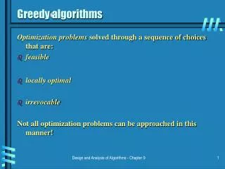
Greedy algorithm’s paradigm Algorithm is greedy if : • it builds up a solution in small consecutive steps • it chooses a decision at each step myopically to optimize some underlying criterion Analyzing optimal greedy algorithms by showing that: • in every step it is not worse than any other algorithm, or • every algorithm can be gradually transformed to the greedy one without hurting its quality Greedy Algorithms and Dynamic Programming
Interval scheduling Input: set of intervals on the line, represented by pairs of points (ends of intervals) Output: the largest set of intervals such that none two of them overlap Generic greedy solution: • Consider intervals one after another using some rule Greedy Algorithms and Dynamic Programming
Rule 1 Select the interval that starts earliest (but is not overlapping the already chosen intervals) Underestimated solution! optimal algorithm Greedy Algorithms and Dynamic Programming
Rule 2 Select the shortest interval (but not overlapping the already chosen intervals) Underestimated solution! optimal algorithm Greedy Algorithms and Dynamic Programming
Rule 3 Select the interval intersecting the smallest number of remaining intervals (but still is not overlapping the already chosen intervals) Underestimated solution! optimal algorithm Greedy Algorithms and Dynamic Programming
Rule 4 Select the interval that ends first (but still is not overlapping the already chosen intervals) Hurray! Exact solution! Greedy Algorithms and Dynamic Programming
Analysis - exact solution Algorithm gives non-overlapping intervals: obvious, since we always choose an interval which does not overlap the previously chosen intervals The solution is exact: Let: • A be the set of intervals obtained by the algorithm, • Opt be the largest set of pairwise non-overlapping intervals We show that A must be as large as Opt Greedy Algorithms and Dynamic Programming
Analysis - exact solution cont. Let A = {A1,…,Ak} and Opt = {B1,…,Bm} be sorted. By definition of Opt we have km. Fact: for every ik, Ai finishes not later than Bi. Proof: by induction. For i = 1 by definition of the first step of the algorithm. From i -1 to i : Suppose that Ai-1 finishes not later than Bi-1. From the definition of a single step of the algorithm, Ai is the first interval that finishes after Ai-1 and does not overlap it. If Bifinished before Ai then it would overlap some of the previous A1,…, Ai-1 and consequently - by the inductive assumption - it would overlap or end before Bi-1, which would be a contradiction. Bi-1 Bi Ai Ai-1 Greedy Algorithms and Dynamic Programming
Analysis - exact solution cont. Theorem:A is the exact solution. Proof: we show that k=m. Suppose to the contrary that k<m. We already know that Ak finishes not later than Bk. Hence we could add Bk+1 to A and obtain a bigger solution by the algorithm - a contradiction. Bk-1 Bk Bk+1 Ak Ak-1 algorithm finishes selection Greedy Algorithms and Dynamic Programming
Implementation & time complexity Efficient implementation: • Sort intervals according to the right-most ends • For every consecutive interval: • If the left-most end is after the right-most end of the last selected interval then we select this interval • Otherwise we skip it and go to the next interval Time complexity: O(n log n + n) = O(n log n) Greedy Algorithms and Dynamic Programming
Textbook and Exercises READING: • Chapter 4 “Greedy Algorithms”, Section 4.1 EXERCISE: • All Interval Scheduling problem from Section 4.1 Greedy Algorithms and Dynamic Programming
Minimum spanning tree Greedy Algorithms and Dynamic Programming
Greedy algorithm’s paradigm Algorithm is greedy if : • it builds up a solution in small consecutive steps • it chooses a decision at each step myopically to optimize some underlying criterion Analyzing optimal greedy algorithms by showing that: • in every step it is not worse than any other algorithm, or • every algorithm can be gradually transformed to the greedy one without hurting its quality Greedy Algorithms and Dynamic Programming
Minimum spanning tree Input: weighted graph G = (V,E) • every edge in E has its positive weight Output: spanning tree such that the sum of weights is not bigger than the sum of weights of any other spanning tree Spanning tree: subgraph with • no cycle, and • spanning and connected (every two nodes in V are connected by a path) 2 2 2 1 1 1 1 1 1 2 2 2 3 3 3 Greedy Algorithms and Dynamic Programming
Properties of minimum spanning trees MST Properties of spanning trees: • n nodes • n - 1 edges • at least 2 leaves (leaf - a node with only one neighbor) MST cycle property: • after adding an edge we obtain exactly one cycle and each edge from MST in this cycle has no bigger weight than the weight of the added edge 2 2 1 1 1 1 cycle 2 2 3 3 Greedy Algorithms and Dynamic Programming
Crucial observation about MST Consider sets of nodes A and V - A • Let F be the set of edges between A and V - A • Let abe the smallest weight of an edge in F Theorem: Every MST must contain at least one edge of weight a from set F A A 2 2 1 1 1 1 2 2 3 3 Greedy Algorithms and Dynamic Programming
Proof of the Theorem Let e be the edge in F with the smallest weight - for simplicity assume that such edge is unique. Suppose to the contrary that e is not in some MST. Consider one such MST. Add e to MST - a cycle is obtained, in which e has weight not smaller than any other weight of edge in this cycle, by the MST cycle property. Since the two ends of e are in different sets A and V - A, there is another edge f in the cycle and in F. By definition of e, such f must have a bigger weight than e, which is a contradiction. A A 2 2 1 1 1 1 2 2 3 3 Greedy Algorithms and Dynamic Programming
Greedy algorithms finding MST Kruskal’s algorithm: • Sort all edges according to their weights • Choose n - 1 edges, one after another, as follows: • If a new added edge does not create a cycle with previously selected edges then we keep it in (partial) solution; otherwise we remove it Remark: we always have a partial forest 2 2 2 1 1 1 1 1 1 2 2 2 3 3 3 Greedy Algorithms and Dynamic Programming
Greedy algorithms finding MST Prim’s algorithm: • Select an arbitrary node as a root • Choose n - 1 edges, one after another, as follows: • Consider all edges which are incident to the currently build (partial) solution and which do not create a cycle in it, and select one having the smallest weight Remark: we always have a connected partial tree root 2 2 2 1 1 1 1 1 1 2 2 2 3 3 3 Greedy Algorithms and Dynamic Programming
Why the algorithms work? Follows from the crucial observations: Kruskal’s algorithm: • Suppose we add edge {v,w}; • This edge has a smallest weight among edges between the set of nodes already connected with v (by a path in already selected subgraph) and other nodes Prim’s algorithm: • Always chooses an edge with a smallest weight among edges between the set of already connected nodes and free nodes (i.e., non-connected nodes) Greedy Algorithms and Dynamic Programming
Time complexity There are implementations using • Union-find data structure (Kruskal’s algorithm) • Priority queue (Prim’s algorithm) achieving time complexity O(m log n) where n is the number of nodes and m is the number of edges in a given graph G Greedy Algorithms and Dynamic Programming
Textbook and Exercises READING: • Chapter 4 “Greedy Algorithms”, Section 4.5 EXERCISES: • Solved Exercise 3 from Chapter 4 • Generalize the proof of the Theorem to the case where may be more than one edges of smallest weight in F Greedy Algorithms and Dynamic Programming
Priority Queues (PQ) Implementation of Prim’s algorithm using PQ Greedy Algorithms and Dynamic Programming
Minimum spanning tree Input: weighted graph G = (V,E) • every edge in E has its positive weight Output: spanning tree such that the sum of weights is not bigger than the sum of weights of any other spanning tree Spanning tree: subgraph with • no cycle, and • connected (every two nodes in V are connected by a path) 2 2 2 1 1 1 1 1 1 2 2 2 3 3 3 Greedy Algorithms and Dynamic Programming
Crucial observation about MST Consider sets of nodes A and V - A • Let F be the set of edges between A and V - A • Let abe the smallest weight of an edge in F Theorem: Every MST must contain at least one edge of weight a from set F A A 2 2 1 1 1 1 2 2 3 3 Greedy Algorithms and Dynamic Programming
Greedy algorithm finding MST Prim’s algorithm: • Select an arbitrary node as a root • Choose n - 1 edges, one after another, as follows: • Consider all edges which are incident to the currently build (partial) solution and which do not create a cycle in it, and select one which has the smallest weight Remark: we always have a connected partial tree root 2 2 2 1 1 1 1 1 1 2 2 2 3 3 3 Greedy Algorithms and Dynamic Programming
Priority queue Set of n elements, each has its priority value (key) • the smaller key the higher priority the element has Operations provided in time O(log n): • Adding new element to PQ • Removing an element from PQ • Taking element with the smallest key Greedy Algorithms and Dynamic Programming
Implementation of PQ based on heaps 2 Heap: rooted (almost) complete binary tree, each node has its • value • key • 3 pointers: to the parent and children (or nil(s) if parent or child(ren) not available) Required property: in each subtree the smallest key is always in the root 4 3 7 5 6 2 3 4 7 5 6 Greedy Algorithms and Dynamic Programming
Operations on the heap PQ operations: • Add • Remove • Take Additional supporting operation: • Last leaf: Updating the pointer to the rigth-most leaf on the lowest level of the tree, after each operation (take, add, remove) Greedy Algorithms and Dynamic Programming
Construction of the heap Construction: • Start with arbitrary element • Keep adding next elements using add operation provided by the heap data structure (which will be defined in the next slide) Greedy Algorithms and Dynamic Programming
Implementing operations on heap Smallest key element: trivially read from the root Adding new element: • find the next last leaf location in the heap • put the new element as the last leaf • recursively compare it with its parent’s key: • if the element has the smaller key then swap the element and its parent and continue; otherwise stop Remark: finding the next last leaf may require to search through the path up and then down (exercise) Greedy Algorithms and Dynamic Programming
Implementing operations on heap Removing element: • remove it from the tree • move the value from last leaf on its place • update the last leaf • compare the moved element recursively either • “up” if its value is smaller than its current parent: swap the elements and continue going up until reaching smaller parent or the root, or • “down” if its value is bigger than its current parent: swap it with the smallest of its children and continue going down until reaching a node with no smaller child or a leaf Greedy Algorithms and Dynamic Programming
Examples - adding 2 2 3 4 3 1 7 5 6 1 7 5 6 4 add 1 at the end swap 1 and 4 2 3 4 7 5 6 1 2 3 1 7 5 6 4 1 3 2 1 3 2 7 5 6 4 swap 1 and 2 Greedy Algorithms and Dynamic Programming 7 5 6 4
Examples - removing 2 6 3 3 4 3 4 6 4 7 5 6 7 5 7 5 remove 2 and swap 6 and 3 removing 2 swap 2 and last element 2 3 4 7 5 6 6 3 4 7 5 3 6 4 7 5 3 5 4 swap 6 and 5 3 5 4 7 6 Greedy Algorithms and Dynamic Programming 7 6
Heap operations - time complexity • Taking minimum: O(1) • Adding: • Updating last leaf: O(log n) • Going up with swaps through (almost) complete binary tree: O(log n) • Removing: • Updating last leaf: O(log n) • Going up or down (only once direction is selected) doing swaps through (almost) complete binary tree: O(log n) Greedy Algorithms and Dynamic Programming
Prim’s algorithm - time complexity Input: graph is given as an adjacency list • Select a root node as an initial partial tree • Construct PQ with all edges incident to the root (weights are keys) • Repeat until PQ is empty • Take the smallest edge from PQ and remove it • If exactly one end of the edge is in the partial tree then • Add this edge and its other end to the partial tree • Add to PQ all edges, one after another, which are incident to the new node and remove all their copies from graph representation Time complexity: O(m log n) where n is the number of nodes, m is the number of edges Greedy Algorithms and Dynamic Programming
Textbook and Exercises READING: • Chapters 2 and 4, Sections 2.5 and 4.5 EXERCISES: • Solved Exercises 1 and 2 from Chapter 4 • Prove that a spanning tree of an n - node graph has n - 1 edges • Prove that an n - node connected graph has at least n - 1 edges • Show how to implement the update of the last leaf in time O(log n) Greedy Algorithms and Dynamic Programming
Dynamic programming Two problems: • Weighted interval scheduling • Sequence alignment Greedy Algorithms and Dynamic Programming
Dynamic Programming paradigm Dynamic Programming (DP): • Decompose the problem into series of sub-problems • Build up correct solutions to larger and larger sub-problems Similar to: • Recursive programming vs. DP: in DP sub-problems may strongly overlap • Exhaustive search vs. DP: in DP we try to find redundancies and reduce the space for searching • Greedy algorithms vs. DP: sometimes DP orders sub-problems and processes them one after another Greedy Algorithms and Dynamic Programming
(Weighted) Interval scheduling (Weighted) Interval scheduling: Input: set of intervals (with weights) on the line, represented by pairs of points - ends of intervals Output: the largest (maximum sum of weights) set of intervals such that none two of them overlap Greedy algorithm doesn’t work for weighted case! Greedy Algorithms and Dynamic Programming
Example Greedy algorithm: • Repeatedly select the interval that ends first (but still not overlapping the already chosen intervals) Exact solution of unweighted case. weight 1 weight 3 weight 1 Greedy algorithm gives total weight 2 instead of optimal 3 Greedy Algorithms and Dynamic Programming
Basic structure and definition • Sort the intervals according to their right ends • Define function p as follows: • p(1) = 0 • p(i) is the number of intervals which finish before ith interval starts p(1)=0 weight 1 p(2)=1 weight 3 p(3)=0 weight 2 weight 1 p(4)=2 Greedy Algorithms and Dynamic Programming
Basic property • Let wj be the weight of jth interval • Optimal solution for the set of first j intervals satisfies OPT(j) = max{ wj + OPT(p(j)) , OPT(j-1) } Proof: If jth interval is in the optimal solution O then the other intervals in O are among intervals 1,…,p(j). Otherwise search for solution among firstj-1 intervals. p(1)=0 weight 1 p(2)=1 weight 3 p(3)=0 weight 2 weight 1 p(4)=2 Greedy Algorithms and Dynamic Programming
Sketch of the algorithm • Additional array M[0…n] initialized by 0,p(1),…,p(n) ( intuitively M[j] stores optimal solution OPT(j) ) Algorithm • For j = 1,…,n do • Read p(j) = M[j] • Set M[j] := max{ wj + M[p(j)] , M[j-1] } p(1)=0 weight 1 p(2)=1 weight 3 p(3)=0 weight 2 weight 1 p(4)=2 Greedy Algorithms and Dynamic Programming
Complexity of solution Time: O(n log n) • Sorting: O(n log n) • Initialization of M[0…n] by 0,p(1),…,p(n): O(n log n) • Algorithm: n iterations, each takes constant time, total O(n) Memory: O(n) - additional array M p(1)=0 weight 1 p(2)=1 weight 3 p(3)=0 weight 2 weight 1 p(4)=2 Greedy Algorithms and Dynamic Programming
Sequence alignment problem Popular problem from word processing and computational biology • Input: two words X = x1x2…xn and Y = y1y2…ym • Output: largest alignment Alignment A: set of pairs (i1,j1),…,(ik,jk) such that • If (i,j) in A then xi = yj • If (i,j) is before (i’,j’) in A then i < i’ and j < j’ (no crossing matches) Greedy Algorithms and Dynamic Programming
Example • Input: X = c t t t c t c c Y = t c t t c c Alignment A: X = c t t t c t c c | | | | | Y = t c t t c c Another largest alignment A: X = c t t t c t c c | | | | | Y = t c t t c c Greedy Algorithms and Dynamic Programming
Finding the size of max alignment Optimal alignment OPT(i,j) for prefixes of X and Y of lengths i and j respectively: OPT(i,j) = max{ ij + OPT(i-1,j-1) , OPT(i,j-1) , OPT(i-1,j) } where ij equals 1 if xi = yj, otherwise is equal to - Proof: If xi = yj in the optimal solution O then the optimal alignment contains one match (xi , yj) and the optimal solution for prefixes of length i-1 and j-1 respectively. Otherwise at most one end is matched. It follows that either x1x2…xi-1 is matched only with letters from y1y2…ym or y1y2…yj-1 is matched only with letters from x1x2…xn. Hence the optimal solution is either the same as for OPT(i-1,j) or for OPT(i,j-1). Greedy Algorithms and Dynamic Programming