Download
1 / 29
300 likes | 514 Views
Binary Stochastic Fields: Theory and Application to Modeling of Two-Phase Random Media. Effects of Random Heterogeneity of Soil Properties on Bearing Capacity. Steve Koutsourelakis University of Innsbruck George Deodatis Columbia University. Radu Popescu and Arash Nobahar

E N D
Binary Stochastic Fields: Theory and Application to Modeling of Two-Phase Random Media Effects of Random Heterogeneity of Soil Properties on Bearing Capacity Steve Koutsourelakis University of Innsbruck George Deodatis Columbia University Radu Popescu and Arash Nobahar Memorial University George Deodatis Columbia University Presented at “Probability and Materials: From Nano- to Macro-Scale,” Johns Hopkins University, Baltimore, MD. January 5-7, 2005
What is a two-phase medium ? A continuum which consists of two materials (phases) that have different properties. What is a random two-phase medium ? A two-phase medium in which the distribution of the two phases is so intricate that it can only be characterized statistically. Examples: Synthetic: fiber composites, colloids, particulate composites, concrete. Natural: soils, sandstone, wood, bone, tumors.
Characterization of Two-Phase Random Media Through Binary Fields black : phase 1 white : phase 2 j = 1 or 2 Complimentarity Condition: • Binary fields assumed statistically homogeneous • Only one of two phases used to describe medium
Random Fields Description First Order Moments – Volume Fraction Second Order Moments – Autocorrelation Properties of the Autocorrelation • If no long range correlation exists: • Positive Definite (Bochner’s Theorem)
Simulation of Homogeneous Binary Fields based on 1st and 2nd order information Available Methods: 1) Memoryless transformation of homogeneous Gaussian fields (translation fields) (Berk 1991, Grigoriu 1988 & 1995, Roberts 1995) Advantage : Computationally Efficient Disadvantage : Limited Applicability
Simulation of Homogeneous Binary Fields based on 1st and 2nd order information Available Methods: 2) Yeong and Torquato 1996 Using a stochastic optimization algorithm, one sample at a time can be generated whose spatial averages match the target. Advantage : Able to incorporate higher order probabilistic information Disadvantage : Computationally costly when a large number of samples needs to be generated
Modeling the Two-Phase Random Medium in 1D Using Zero Crossings are equidistant values of a stationary, Gaussian stochastic process Y(x) with zero mean, unit variance and autocorrelation medium
Modeling the Two-Phase Random Medium in 1D is also statistically homogeneous with autocorrelation 2nd order joint Gaussian p.d.f Observe that:
Modeling the Two-Phase Random Medium in 1D Observe that: For any pair , the correlation matrix : is always positive definite
Modeling the Two-Phase Random Medium in 1D 4th order joint Gaussian p.d.f The function H doesn’t have an explicit form, except for special cases. It can be calculated numerically with great computational efficiency (Genz 1992).
Three Gaussian Autocorrelations Corresponding Binary Autocorrelations
case 1 – strong clustering case 2– medium clustering case 3 – weak clustering Sample Realizations of Three Cases with Different Clustering (but same )
Simulation: Inversion Algorithm For simulation purposes, the inverse path has to be followed. The goal is to find a Gaussian autocorrelation that can produce the target binary autocorrelation • Questions: • Existence of for arbitrary • Uniqueness of Approximate solutions – Optimization Formulation Find Gaussian autocorrelation that produces a binary autocorrelation which minimizes the error with :
Iterative Inversion Algorithm – Basic Concept Step 1: Start with an arbitrary Gaussian autocorrelation such that and . Calculate the binary autocorrelation and the error Step 2: Perturb the values of by small amounts, keeping and the same. Calculate the new and the new error e. If the error is smaller, then keep the changes in otherwise reject them. Step 3: Repeat Step 2 until the error e becomes smaller than a prescribed tolerance of if a large number of iterations do not further reduce the error e.
Example – Known Gaussian Autocorrelation Binary autocorrelation Gaussian autocorrelation Observe stabilityof the mapping
Example – Debye Medium Binary autocorrelation
Example – Debye Medium Gaussian autocorrelation Gaussian Spectral Density Function
Example – Debye Medium Progression of Error Sample Realization
Simulation: Inversion Algorithm Advantage of the Method Proposed: The inversion procedure has to be performed onlyonce. Once the underlying Gaussian autocorrelation is determined, samples of the corresponding Gaussian process can be generated very efficiently using the Spectral Representation Method (Shinozuka & Deodatis 1991). These Gaussian samples are then mapped according to: in order to produce the samples of the binary sequence.
Example – Anisotropic Medium Target Inversion
Example – Anisotropic Medium Gaussian autocorrelation Gaussian Spectral Density Function
Example – Anisotropic Medium Sample Realization
Example – Fontainebleau Sandstone Target Inversion
Example – Fontainebleau Sandstone Gaussian autocorrelation Gaussian Spectral Density Function
Example – Fontainebleau Sandstone Actual Image Simulated Image
Generalized Formulation Consider a homogeneous, zero mean, unit variance, Gaussian random field with autocorrelation: will also be homogeneous
Generalized Formulation Autocorrelation In general:
Generalized Formulation: Discretization in 1D Properties of the Autocorrelation • For we recover the previous formulation • depend on: Surplus of parameters Surplus of parameters makes the method more flexible and able to describe a wider range of binary autocorrelation functions.
Conclusions • The method proposed is shown capable of generating samples of a wide range of binary fields using nonlinear transformations of Gaussian fields. • It takes advantage of existing methods for the generation of Gaussian samples and requires minimum computational cost especially when a large number of samples is needed. • Generalized formulation increases the range of binary fields that can be modeled. • Extension to higher order probabilistic information. • Extension to more than two phases. • Extension to three dimensions.