Download
1 / 55
550 likes | 696 Views
This document explores various probability distributions, including Discrete Uniform, Binomial, Geometric, Poisson, Hypergeometric, Negative Binomial, Continuous Uniform, Normal, and Exponential. For each distribution, it presents real-world examples that illustrate how to calculate probabilities, expected values, and variances. Key questions include the likelihood of specific outcomes, along with comprehensive calculations and interpretations. Perfect for students and professionals seeking to deepen their understanding of probability theory.

E N D
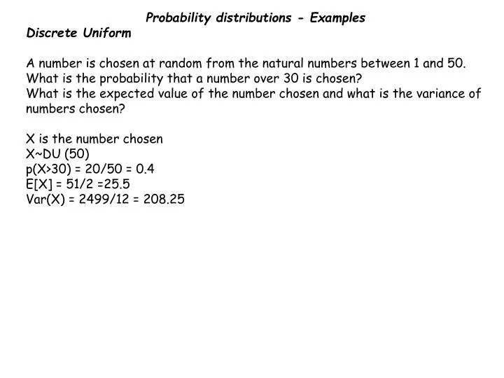
Probability distributions - Examples Discrete Uniform A number is chosen at random from the natural numbers between 1 and 50. What is the probability that a number over 30 is chosen? What is the expected value of the number chosen and what is the variance of numbers chosen? X is the number chosen X~DU (50) p(X>30) = 20/50 = 0.4 E[X] = 51/2 =25.5 Var(X) = 2499/12 = 208.25
Probability distributions - Examples Binomial A marksman fires at a target 10 times, with probability of hitting the target 9/10. What is the probability that he hits the target exactly 8 times? What is the probability that he hits the target more than 6 times? What is the expected value of the number of hits and what is the variance of the number of hits? X is the number of hits X~B(10, 0.9) p(X=8) = 0.194 p(X>6) = 1 – p(X≤6) = 0.987 E[X] = 10x0.9 = 9 Var(X) = 10x0.9x0.1 = 0.9
Probability distributions - Examples Geometric A marksman fires at a target with probability of hitting the target 9/10. What is the probability that he hits the target for the first time on his second shot? What is the probability that he takes at least 5 shots to hit the target for the first time? What is the expected value of the number of shots before he hits the target and what is the variance of the number of shots before hitting the target? X is the number of shots before he hits the target X~Geo(0.9) p(X=2) = 0.09 p(X≥5) = 1 – p(X≤4) = 0.0001 E[X] = 10/9 = 1.11 Var(X) = 0.123
Probability distributions - Examples Poisson It is known that on average the number of people visiting a shop in an hour is 17. What is the probability that exactly 30 people visit the shop in a two hour period? What is the probability that less than 50 people visit the shop in the first three hours of opening? What is the expected number of people visiting the shop in an 8 hour day, and what is the variance of the number of people visiting? X is the number of people visiting in 2 hours X~Po(34) p(X=30) = 0.0568 Y is the number of people visiting in 3 hours Y~Po(51) p(Y<50) = p(Y≤49) = 0.426 Z is the number of people visiting in 8 hours Z~Po(136) E[Z] = 136 Var(Z) = 136
Probability distributions - Examples Hypergeometric There are 20 students studying HL maths, of which 14 are girls. If 8 students from the HL classes are chosen at random to visit the maths department of a particular university, what is the probability that exactly 3 girls are chosen? What is the expected number of girls chosen in the group and what is the variance of the number of girls? X is the number of girls in the group X~Hyp(8,14,20) p(X=3) = 364x6/125970 = 0.0173 E[X] = 5.6 Var(X) = 504/475
Probability distributions - Examples Negative Binomial A marksman fires at a target with probability of hitting the target 9/10. What is the probability that he hits the target for the third time on his eighth shot? What is the expected value of the number of shots before he hits the target for the fifth time and what is the variance? X is the number of shots before he hits the target for the third time X~NB(3,0.9) p(X=8) = 0.000153 Y is the number of shots before he hits the target for the fifth time Y~NB(5,0.9) E[Y] = 50/9 Var(Y) = 50/81
Probability distributions - Examples Continuous Uniform A number is chosen at random from the real numbers between 0 and 50. What is the probability that a number over 30 is chosen? What is the expected value of the number chosen and what is the variance of numbers chosen? X is the number chosen X~U(0,50) p(X>30) = 20/50 = 0.4 E[X] = 50/2 =25 Var(X) = 2500/12 = 208
Probability distributions - Examples Normal The lengths of worms are normally distributed with mean 7.2cm and standard deviation 2.3cm Find the probability that a worm chosen at random is greater than 8cm X is the length of the worm X~N(7.2, 2.32) p(X>8) = 0.364 Another species of worm also have their lengths normally distributed and 40% of worms are longer than 8cm and 20% less than 5cm. Find the mean and standard deviation of the lengths of these worms Y is the length of the worm Y~N(m,s2)p(Y<8) = 0.6, p(Y<5) = 0.2 8 – m = 0.253347s 5 – m = -0.841621s m = 7.31 and s = 2.74 Remember Z = (Y – m)/s So (Y – m)/s = F-1(0.6)
Probability distributions - Examples Exponential It is known that on average the number of people visiting a shop in an hour is 18. If there is no-one in the shop at present, find the probability that it is more than 10 minutes before someone comes into the shop. Find the expected amount of time before someone comes into the shop and the variance of that time. X is the amount of time before someone comes into the shop X~Exp(0.3) p(X>10) = 0.0498 E[X] = 10/3 Var(X) = 100/9
Expectation Algebra Three coins are tossed and the number of heads is recorded X is the number of heads X ~ B(3, 0.5) Two dice are thrown and the number of sixes recorded Y is the number of sixes Y ~ B(2, 1/6)
E[X] = 3/2 and Var(X) = 3/4 E[Y] = 1/3 and Var(Y) = 5/18 Now what if I want to consider the total number of heads and sixes in the two experiments What will be the expectation and variance for the total? Remember E[X] = np And Var(X) = npq
P(Z = 0) = (1/8)(25/36) = 25/288 P(Z = 1) = (3/8)(25/36)+(1/8)(10/36)=85/288 P(Z = 3) = (1/8)(25/36)+(3/8)(10/36)+(3/8)(1/36) =58/288 P(Z = 2) = (3/8)(25/36)+(3/8)(10/36)+(1/8)(1/36) =106/288 P(Z = 4) = (1/8)(10/36)+(3/8)(1/36) = 13/288 P(Z = 5) = (1/8)(1/36) = 1/288 So E[X + Y] = So E[X + Y] = 11/6 and Var(X + Y) = 37/36 = E[X] + E[Y] = Var(X) + Var(Y)
In general: E[X + Y] = E[X] + E[Y] Var(X + Y) = Var(X) + Var(Y) However more generally E[aX ± bY] = aE[X] ± bE[Y] Var(aX ± bY) = a2Var(X) + b2Var(Y) Note only +
Example 1: The weights of apples are normally distributed with mean 380g and standard deviation 45g and the weights of bananas are normally distributed with mean 240g and standard deviation 25g. A bag contains three apples and 5 bananas. What is the probability that the bag weighs more than 2.5kg? Solution: W = A1 + A2 + A3 + B1 + B2 + B3 + B4 + B5 and Ak~N(380,452), Bk~N(240,252) E[W] = E[A1 + A2 + A3 + B1 + B2 + B3 + B4 + B5] = E[A1] + E[A2] + E[A3] + E[B1] + E[B2] + E[B3] + E[B4] + E[B5] =3 x 380 + 5 x 240 = 2340 Var(W) = Var(A1 + A2 + A3 + B1 + B2 + B3 + B4 + B5) = Var(A1) + Var(A2) + Var(A3) + Var(B1) + Var(B2) + Var(B3) + Var(B4) + Var(B5) =3 x 452 + 5 x 252 = 9200 So W~N(2340, 9200) P(W>2500) = 0.0476
Example 2: The weights of apples are normally distributed with mean 380g and standard deviation 45g and the weights of bananas are normally distributed with mean 240g and standard deviation 25g. Apples cost 3 pesos per gram and bananas cost 5 pesos per gram If I buy an apple and a banana at random, what is the probability I spend more than 2500 pesos? Solution: C = 3A + 5B and A~N(380,452), B~N(240,252) E[C] = E[3A + 5B] = 3E[A] + 5E[B] =3 x 380 + 5 x 240 = 2340 Var(C) = Var(3A + 5B) = 9Var(A) + 25Var(B) =9 x 452 + 25 x 252 = 33850 So W~N(2340, 33850) P(W>2500) = 0.192 Compare this to example 1
Example 3: The weights of apples are normally distributed with mean 380g and standard deviation 45g and the weights of bananas are normally distributed with mean 240g and standard deviation 25g. If I buy an apple and a banana at random, what is the probability that the apple is more than twice as heavy as the banana? Solution: D = A - 2B and A~N(380,452), B~N(240,252) E[D] = E[A - 2B] = E[A] - 2E[B] =380 – 2 x 240 = -100 Var(D) = Var(A - 2B) = Var(A) + 4Var(B) =452 + 4 x 252 = 4525 So D~N(-100, 4525) P(D>0) = 0.0686
The distribution of sample means When making inferences about a POPULATION we usually have to do so from the data provided by a SAMPLE. For example if I want to estimate the number of children per family in Switzerland, I may take a sample of 50 families to make my estimate. Suppose the mean of my sample is 2.6 children per family I can ESTIMATE the mean of the population (all families in Switzerland) to be 2.6 children per family If someone else did the same thing, they would very likely find a different estimate for the mean number of children per family If many people did the same thing, we would have many different sample means. The CENTRAL LIMIT THEOREM states that the distribution of sample means of size n is approximately Normal with mean m and standard deviation where m and s are the mean and standard deviation of the population
The distribution of sample means So The Central Limit Theorem is exact if the sample is from a Normally distributed population, and if it not a Normally distributed population, the Central Limit Theorem still applies as an approximation – the larger the value of n, the better the approximation. We can see that as n increases, so the standard deviation decreases.
Using the Central Limit theorem • Example 1 • On a certain beach, turtles go each year to lay their eggs. • The number of eggs in a nest is known to be normally distributed with mean 114.78 and standard deviation 22.4 • Calculate the probability that the mean number of eggs in a sample of 10 nests is greater than 120 • If a sample of 5 nests is taken, calculate the value of a, such that the probability of the mean of the sample is within a of the mean is 90% • Solution • (a) • (b)
The Proportion of success in a large sample An egg manufacturer claims that eggs delivered to a supermarket have no more than 5% that are broken. On a certain day, of 1000 eggs delivered to the supermarket, 80 are found to be broken. What is the probability of this happening? Briefly comment on the manufacturer’s claim Method 1 – exact X are the number of broken eggs in the delivery X ~ B(1000, 0.05) p(X ≥ 80) = 3.49 × 10⁻⁵ It seems very unlikely that the manufacturer’s claim is correct
The Proportion of success in a large sample Method 2 – Using the central limit theorem X are the number of broken eggs in the delivery X ~ B(1000, 0.05) so E[X] = 50 and Var(X) = 47.5 Now if then and So if n is large (by the Central Limit Theorem)
The Proportion of success in a large sample So in this example So It still seems very unlikely that the manufacturer’s claim is correct. Note that the answer is a little inaccurate due to the approximation of the CLT
The Proportion of success in a large sample This can also be found on the GDC using the 1-proportion Z test On the STAT menu find 1-PropZTest Set and Calculate
The Proportion of success in a large sample Another Example A drug company claims that a new drug cures 75 % of patients suffering from a certain disease. However, a medical committee believes that less than 75 % are cured. To test the drug company’s claim, a trial is carried out in which 100 patients suffering from the disease are given the new drug. It is found that 68 of these patients are cured. Does the medical committee have the evidence it requires to refute the drug company’s claim? Solution We assume 75% of patients are cured by the drug Method 1 Number of patients cured is X X ~ B(100, 0.75) p(X ≤ 68) = 0.0693
The Proportion of success in a large sample Another Example A drug company claims that a new drug cures 75 % of patients suffering from a certain disease. However, a medical committee believes that less than 75 % are cured. To test the drug company’s claim, a trial is carried out in which 100 patients suffering from the disease are given the new drug. It is found that 68 of these patients are cured. Does the medical committee have the evidence it requires to refute the drug company’s claim? Solution Assuming 75% of patients are cured by the drug Method 2
The Proportion of success in a large sample Another Example A drug company claims that a new drug cures 75 % of patients suffering from a certain disease. However, a medical committee believes that less than 75 % are cured. To test the drug company’s claim, a trial is carried out in which 100 patients suffering from the disease are given the new drug. It is found that 68 of these patients are cured. Does the medical committee have the evidence it requires to refute the drug company’s claim? Solution Assuming 75% of patients are cured by the drug Method 3 From GDC using 1-PropZTest p = 0.0530
Hypothesis Testing In the previous example, what could you conclude? Was the drug company’s claim valid? Would the medical committee have sufficient evidence for a lawsuit? We need to develop a more formal approach to testing the hypothesis First we write the hypothesis in a formal way. We say that the NULL HYPOTHESIS is that the company’s claim is correct – i.e. that 75% of patients are cured Also the ALTERNATIVE HYPOTHESIS is that LESS than 75% are cured Note that we are not interested in this case if MORE than 75% are cured This is called a 1-TAIL TEST
Hypothesis Testing We write: H0: 75% of patients cured by the drug H1: Less than 75% of patients cured by the drug OR H0: p=0.75 H1: p<0.75
Hypothesis Testing H0: p=0.75 H1: p<0.75 Now we can find the probability of the result found as before (by any of the methods) Next we decide on a SIGNIFICANCE LEVEL If we need to be very sure (e.g. to take out a lawsuit) then we need a low significance level. A higher level if it is not so important Note that you will usually be given the significance level Usually it is 10%, 5%, or 1%
Hypothesis Testing H0: p=0.75 H1: p<0.75 So if we test at the 10% level (probably not sure enough for a lawsuit) Then as 5.3% < 10%, we would reject H0 in favour of H1. The company’s claim does not seem reasonable On the other hand if we test at the 1% level Then as 5.3% > 1%, there is insufficient evidence to reject H0 and we accept the company’s claim that 75% of patients are cured by the drug
Hypothesis Testing In the previous example the standard deviation was known, as the distribution of number of patients etc. was Binomial. In other cases, the standard deviation may be known (by other sources) or estimated from the sample. These cases give rise to different types of hypothesis testing
Hypothesis Testing • For example • A sample of 10 crates of items is taken from a factory which states that the mean number of defective items per crate is 12. The sample mean of the ten crates is found to be 13. Knowing that the standard deviation of the number of defective items is 1.6, test the hypothesis that the mean is more than 12: • at the 10% level of significance • (b) at the 1% level of significance
Hypothesis Testing H0: m = 12 H1: m > 12 by the central limit theorem (a) so testing at the 10% level of significance we see that 2.5%<10% so we reject H0 in favour of H1, the mean number of defective items is greater than 12 (b) testing at the 1% level of significance we see that 2.5%>1% so there is insufficient evidence to reject H0. We accept that the manufacturer’s claim that the mean number of defective items is 12
Hypothesis Testing Or! H0: m = 12 H1: m > 12 (a) so testing at the 10% level of significance we see that 2.5%<10% so we reject H0 in favour of H1, the mean number of defective items is greater than 12 (b) testing at the 1% level of significance we see that 2.5%>1% so there is insufficient evidence to reject H0. We accept that the manufacturer’s claim that the mean number of defective items is 12
Hypothesis Testing Another example A sample of 5 crates of items is taken from a factory which states that the mean number of defective items per crate is 12. The sample is 12, 13, 11, 14, 13. Knowing that the standard deviation of the number of defective items is 1.6, test the hypothesis at the 5% level of significance Solution H0: m = 12 H1: m > 12 Sample mean is 12.6 (from GDC) 20%>5% so there is insufficient evidence to reject H0. We accept that the mean number of defective items is 12 Or from GDC using Z-Test
Hypothesis Testing Now if the standard deviation of the population is NOT known, and has to be estimated from the sample, then the distribution is altered. Rather than being Normal, the distribution follows that of a Student-t distribution. The standardised Student-t distribution has parameter u, known as the degrees of freedom The degrees of freedom is generally n - 1
Hypothesis Testing • For example • A sample of 10 crates of items is taken from a factory which states that the mean number of defective items per crate is 12. The sample mean of the ten crates is found to be 13 and the estimate of the standard deviation of the number of defective items is 1.6, test the hypothesis that the mean is more than 12: • at the 10% level of significance • (b) at the 1% level of significance
Hypothesis Testing H0: m = 12 H1: m > 12 (a) so testing at the 10% level of significance we see that 3.98%<10% so we reject H0 in favour of H1, the mean number of defective items is greater than 12 (b) testing at the 1% level of significance we see that 3.98%>1% so there is insufficient evidence to reject H0. We accept that the manufacturer’s claim that the mean number of defective items is 12 Note the degrees of freedom is 9 and S is the estimate of the population standard deviation Or use T-Test on the GDC
Hypothesis Testing Error Types Falsely rejecting H0, is known as a Type I error Falsely accepting H0, is known as a Type II error So in the example used previously: ..testing at the 10% level of significance we see that 2.5%<10% so we reject H0 in favour of H1, the mean number of defective items is greater than 12. There is a 2.5% risk of committing a type I error
Confidence intervals A confidence interval is an interval in which we are certain to a given probability of the mean lying in that interval. For example if a 95% confidence interval is given, then there would be a 95% probability that the mean is in that interval. Example 1 On a given busy day, 1000 eggs are delivered to a supermarket and 80 are broken. Find the 95% confidence interval for the mean percentage of broken eggs.
Confidence intervals Example 1 On a given busy day, 1000 eggs are delivered to a supermarket and 80 are broken. Find the 95% confidence interval for the mean percentage of broken eggs. Method 1 As before We can estimate p as 0.08 so Now if Then so and the confidence interval is [6.32%, 9.68 %]
Confidence intervals Example 1 On a given busy day, 1000 eggs are delivered to a supermarket and 7% are broken. Find the 95% confidence interval for the mean percentage of broken eggs. Method 2 From formula book For a 95% confidence interval we take z=InvNorm(0.975)=1.96 So applying the formula we find the confidence interval to be [6.32%, 9.68%] Method 3 From GDC using 1-PropZInt, the interval is [6.32%, 9.68%]
Confidence intervals Example 2 To test a drug company’s claim, a trial is carried out in which 100 patients suffering from a disease are given a new drug. It is found that 68 of these patients are cured. Find a 90% confidence interval for the proportion of patients cured by the drug. Method 1 a = 0.0767 So the confidence interval is [0.603, 0.757] Or either of the other two methods!
Example 3 • A sample of 10 crates of items is taken from a factory and the mean of the ten crates is found to be 13. Knowing that the standard deviation of the number of defective items is 1.6, find a 95% confidence interval for the mean number of defective items in a crate. • Solution • So the confidence interval is [12.01, 13.99] • Or use the formula in the formula book • Or use ZInterval on the GDC
Confidence intervals Again if the standard deviation of the population is NOT known, and has to be estimated from the sample, then the distribution is altered to that of a Student-t distribution.
Example 4 A sample of 10 crates of items is taken from a factory and the sample mean of the ten crates is found to be 13 and the estimate of the standard deviation of the number of defective items is 1.6. Find a 90% confidence interval for the mean number of defective items. Solution As before so a = 0.927 (1.833 × 1.6 / 10) (from tables or solver) So the confidence interval is [12.07, 13.93] • Or use the formula in the formula book • Or use TInterval on the GDC
The 2– Goodness of fit test A dice is thrown 60 times and the following frequencies are obtained Score 1 2 3 4 5 6 Frequency 12 13 10 11 11 3 Is there evidence to suggest that the dice is biased? How can we calculate the probability of results as extreme as these in order to test a hypothesis? We use the fact that the quantity approximately follows a 2 probability distribution Note that if any of the expected frequencies are less than 5, then the chi-squared distribution may not be a reasonable approximation
The 2– Goodness of fit test So following standard hypothesis testing procedures H0: the dice is fair – i.e. X~UD(6) where X is the score H1: the dice is biased – i.e. the distribution is not uniform So taking u = 5 So testing at the 5% significance level, 27%>5% so there is insuficient evidence to reject H0. We accept that the dice is not biased. Also this can be done on a TI84
More on Degrees of freedom • = no of classes – no of restrictions – no of estimated parameters So often u = n – 1 as there is a restriction on the total frequency (as in the previous example)