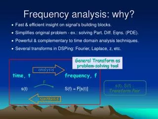
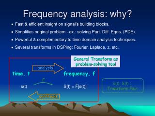
Frequency analysis: why?
analysis. General Transform as problem-solving tool. s(t), S(f) : Transform Pair. time, t frequency, f F s(t) S(f) = F [s(t)]. synthesis. Frequency analysis: why?. Fast & efficient insight on signal’s building blocks. Simplifies original problem - ex.: solving Part. Diff. Eqns. (PDE).

Frequency analysis: why?
E N D
Presentation Transcript
analysis General Transform as problem-solving tool s(t), S(f) : Transform Pair time, tfrequency, f F s(t) S(f) = F[s(t)] synthesis Frequency analysis: why? • Fast & efficient insight on signal’s building blocks. • Simplifies original problem - ex.: solving Part. Diff. Eqns. (PDE). • Powerful & complementary to time domain analysis techniques. • Several transforms in DSPing: Fourier, Laplace, z, etc.
Fourier analysis - applications • Applications wide ranging and ever present in modern life • Telecomms - GSM/cellular phones, • Electronics/IT - most DSP-based applications, • Entertainment - music, audio, multimedia, • Imaging, image processing, • Industry/research - X-ray spectrometry, chemical analysis (FT spectrometry), radar design, • Medical - EGG, heart malfunction diagnosis, • Speech analysis (voice activated “devices”, biometry, …).
Periodic (period T) FS Discrete Continuous Aperiodic FT Continuous ** Periodic (period T) DFS Discrete Discrete DTFT Continuous Aperiodic ** DFT Discrete ** Calculated via FFT Note: j =-1, = 2/T, s[n]=s(tn), N = No. of samples Fourier analysis - tools Input Time Signal Frequency spectrum
A periodic function s(t) satisfying Dirichlet’s conditions * can be expressed as a Fourier series, with harmonically related sine/cosine terms. a0, ak, bk : Fourier coefficients. k: harmonic number, T: period, = 2/T For all t but discontinuities (signal average over a period, i.e. DC term & zero-frequency component.) * see next slide Fourier Series (FS) synthesis analysis Note: {cos(kωt), sin(kωt) }k form orthogonal base of function space.
FS synthesis Square wave reconstruction from spectral terms Convergence may be slow (~1/k) - ideally need infinite terms. Practically, series truncated when remainder below computer tolerance ( error). BUT … Gibbs’ Phenomenon.
Gibbs phenomenon Overshoot exist @ each discontinuity
FourierIntegral Theorem Any aperiodic signal s(t) can be expressed as a Fourier integral if s(t) piecewise smooth(1) in any finite interval (-L,L) and absolute integrable(2). s(t) continuous, s’(t) monotonic (1) (3) (2) (3) Complex form Real-to-complex link Fourier Transform (Pair) - FT synthesis analysis Fourier Integral (FI) Fourier analysis tools for aperiodic signals.
S(f) = 2 sMAX sync(2f) Power Spectral Density (PSD) vs. frequency f plot. Note: Phases unimportant! FT - example FT of 2-wide square window
3 Integer part Fractional part Early computers (ex: ENIAC) mainly base-10 machines. Mostly turned binary in the ’50s. a) less complex arithmetic h/w; Benefits b) less storage space needed; c) simpler error analysis. Digital data formats Positional number system with baseb: [ .. a2 a1 a0.a-1 a-2 .. ]b = .. + a2 b2 + a1 b1 + a0 b0 + a-1 b-1 + a-2 b-2+ .. Important bases: 10 (decimal), 2 (binary), 8 (octal), 16 (hexadecimal).
3 Ex: 3-bit formats 15 14 ... 0 Unsigned integer Offset-Binary Sign-Magnitude Two’s complement 7111 4111 3011 3 011 6110 3110 2010 2010 MSB LSB 5101 2101 1001 1001 4100 1100 0000 0000 Fractional point (DSPs) 3011 0011 0100 -1111 2010 -1010 -1101 -2110 1001 -2001 -2110 -3101 Sign bit 0000 -3000 -3111 -4100 Decimal equivalent Binary representation Fixed-point binary Represent integer or fractional binary numbers. NB: Constant gap between numbers.
3 31 30 23 22 0 Precision e s f MSB LSB Single (32 bits) Double (64 bits) Double-extended ( 80 bits) e = exponent, offset binary, -126 < e < 127 s = sign, 0 = pos, 1 = neg f = fractional part, sign-magnitude + hidden bit Single precision range Max = 3.4 · 1038 Min = 1.175 · 10-38 Coded number x = (-1)s · 2e · 1.f NB: Variable gap between numbers. Large numbers large gaps; small numbers small gaps. Floating-point binary - 2 IEEE 754 standard
3 Overflow : arises when arithmetic operation result has one too many bits to be represented in a certain format. largest value smallest value Fixed point ~ 180 dB Floating point ~1500 dB Dynamic rangedB= 20 log10 High dynamic range wide data set representation with no overflow. NB: Different applications have different needs. Ex: telecomms: 50 dB; audio: 90 dB. Finite word-length effects
DSP Devices & Architectures • Selecting a DSP – several choices: • Fixed-point; • Floating point; • Application-specific devices(e.g. FFT processors, speech recognizers,etc.). • Main DSP Manufacturers: • Texas Instruments (http://www.ti.com) • Motorola (http://www.motorola.com) • Analog Devices (http://www.analog.com)
Pseudo C code for (n=0; n<N; n++) { s=0; for (i=0; i<L; i++) { s += a[i] * x[n-i]; } y[n] = s; } Typical DSP Operations • Filtering • Energy of Signal • Frequency transforms
Traditional DSP Architecture X RAM Y RAM a x(n-i) Multiply/Accumulate Accumulator y(n) Most modern DSPs have more advanced features.
‘C5000 (‘C54x) ‘C5x ‘C2000 (‘C20x, ‘C24x) ‘C1x ‘C2x TI’s DSP Portfolio ‘C6000 (‘C62x, ‘C67x) • Power Efficient Performance • Wireless Telephones/IADs • Modems / Telephony • VoIP • .32ma/MIPS to sub 1V parts • $5 / 100 MIPS ‘C3x ‘C4x ‘C8x • Control Efficient • Storage • Brushless Motor Control • Flash Memory • A/D • PWM Generators • High Performance • Multi-Channel / Function • Comm Infrastructure • xDSL • Imaging, Video • VLIW architecture • 2400 MIPS + • Roadmap to 1 GHZ
PAST PRESENT C5000 TRANSFORMS QUALITY OF LIFE Past Present Cellular Phones Bulky Sleek, Compact Short Battery Life Lasting Performance Programmable, Multi-function A Few, Fixed Functions Internet Audio Supports Multiple Standards, Field Upgradable Supports One Standard Long Design Cycle Fast Design Cycle Digital Cameras Personal and Portable Applications