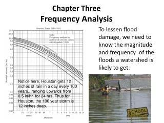
Challenges in Frequency Analysis of Hydrological Data: Extrapolation and Data Limitations
This document delves into critical issues faced during frequency analysis of hydrological data, including extrapolation errors, short recording periods, and the handling of extreme and non-extreme data. It emphasizes the importance of data stationarity and accuracy, noting that misclassifications can lead to severe mispredictions in flood events. The limitations of gauge coverage and routing are discussed, highlighting the necessity of robust statistical methods and proper verification of results to ensure reliable flood risk assessments.

Challenges in Frequency Analysis of Hydrological Data: Extrapolation and Data Limitations
E N D
Presentation Transcript
Problems 1. Extrapolation 2. Short Records 3. Extreme Data 4. Non-extreme Data 5. Stationarity of Data 6. Data Accuracy 7. Peak Instantaneous Data 8. Gauge Coverage 9. No Routing 10. No Correct Distribution 11. Variation In Results 12. No Verification Of Results 13. Mathematistry
1. Extrapolation • Danger in fitting to known set of data and extrapolating to the unknown, without understanding physics • Example of US population growth chart : • Tight fit with existing data • Application of “accepted” distribution • No understanding of underlying factors • Results totally wrong
1. Extrapolation US Population Extrapolation Thompson (1942) reported in Klemes (1986)
2. Short Records • Ideally require record length several times greater than desired return period • Alberta has over 1000 gauges with records, but very few are long • Frequency analysis results can be very sensitive to addition of one or two data points • Subsampling larger records indicates sensitivity
3. Extreme Data • The years recorded at a gauge may or may not have included extreme events • Large floods known to have occurred at gauge sites but not recorded • Some gauges may have missed extreme events only by chance e.g. 1995 flood - originally predicted for Red Deer basin, but ended up on the Oldman basin. The Red Deer and Bow River basins have not seen extreme floods in 50 to 70 years • Presence of several extreme events could cause frequency analysis to over-predict • Presence of no extreme events could cause frequency analysis to under-predict
3. Extreme Data Gauge 05BH004 Bow River At Calgary
3. Extreme Data Gauge 05BH004 Bow River At Calgary
4. Non-extreme Data • All data points are used by statistical methods to fit a distribution. Most of these points are for non-extreme events, that have very different physical responses than extreme events e.g. : • magnitude, duration, and location of storm • snowmelt vs. rainfall • amount of contributing drainage area • initial moisture • impact of routing at lower volumes of runoff • Fitting to smaller events may cause poor fit and extrapolation for larger events • Impact of change in values at left tail impact the extrapolation on the right - makes no physical sense
4. Non-extreme Data Gauge 05BH004 Bow River At Calgary
4. Non-extreme Data A - Original Fit B - 3 lowest points slightly reduced C - 3 lowest points slightly increased East Humber River, Ontario Klemes (1986)
5. Stationarity Of Data • Changes may have occurred in basin that affect runoff response during the flow record e.g. • man-made structures - dams, levees, diversions • land use changes - agriculture, forestation, irrigation • In order to keep the equivalent length of record, hydrologic modelling would be required to convert the data so that it would be consistent. • This modelling would be very difficult as it it would cover a wide range of events over a number of years
6. Data Accuracy • Extreme data often not gauged • Extrapolated using rating curves • Channel changes during large floods - geometry, roughness, sediment transport, • Problems with operation of stage recording gauges e.g. damage, ice effects • Problems with data reporting e.g. Fish Ck, 1915 • Hydrograph examination can ID problems
6. Data Accuracy Highest Recorded Water Level Highest Gauge Measurement Gauge 05AA004 Pincher Ck - 1995
6. Data Accuracy • Qi reported as 200 m3/s • Does not fit mean daily flows Gauge 05BK001 Fish Ck - 1915
7. Peak Instantaneous Data • Design discharge is based on peak instantaneous values, but sometimes this data is not available • Conversion of mean daily data to instantaneous requires consideration of the hydrograph timing e.g. peaks near midnight vs. peaks near noon • Different storm durations can result in very different peak to mean daily ratios for the same basin • Applying a multiplier to the results of a frequency analysis based on mean daily values can lead to misleading results • Statistical methods require that all data points be consistent, even though many are irrelevant to extrapolation
7. Peak Instantaneous Data Gauge 05AA023 Oldman R - 1995
7. Peak Instantaneous Data Oldman R Dam
8. Gauge Coverage • Limited number of gauges in province with significant record lengths • Difficult to transfer peak flow number to other sites without consideration of hydrographs and routing • Area exponent method very sensitive to assumed number
All Gauges (1085) Gauges >30 Years (212) 8. Gauge Coverage
9. No Routing • Peak instantaneous flow value is only applicable at the gauge site • Need hydrograph to rout flows, not just peak discharges • Major Routing Factors include : • Basin configuration • Lakes and reservoirs • Floodplain storage • inter-basin transfers e.g. Highwood - Little Bow River
15 10 5 0 0 20 40 60 80 9. No Routing Inflow Outflow Discharge (m3/s) Time (hrs)
10. No Correct Distribution • Application of theoretical probability distributions and fitting techniques originated with Hazen (1914) in order to make straight line extrapolations from data • There is no reason why they should be applicable to hydrologic observations • None of them can account for the physics of the site during extrapolation • discharge limits due to floodplain storage • addition of flow from inter-basin transfer at extreme events • changes in contributing drainage area at extreme events
11. Variation in Results • Different distributions and fitting techniques can yield vastly different results • Many distributions in use - LN2, LN3, LP3, GEV, P3 • Many fitting techniques - Moments, Maximum Likelihood, Least Squares Fit, PWM • No way to distinguish between which one is the most appropriate for extrapolation • Extrapolated values can be physically unrealistic
11. Variation in Results Gauge 05AD003 Waterton River Near Waterton 74 Years of Record
11. Variation in Results Gauge 05BL027 Trap Ck Near Longview 20 Years of Record
12. No Verification Of Results • Due to the separation of frequency analysis from physical modelling, the process cannot be tested. • 1:100 year flood predictions cannot be actually tested for 100's or 1000's of years. • There is therefore little opportunity to refine an analysis or to improve confidence in its applicability
13. Mathematistry • Gain artificial confidence in accuracy due to mathematical precision • statistics - means, standard deviations, skews, kurtosis, outliers, confidence limits • curve fitting - moments, max likelihood, least squares, probability weighted moments • probability distributions - LN3, LP3, GEV, Wakeby • Loose sight of physics with focus on numbers
Conclusions • Statistical frequency analysis has many problems in application to design discharge estimation for bridges. • If frequency analysis is to be employed, extrapolation should be based on extreme events. This can be accomplished using graphical techniques if appropriate data exists. • Alternative approaches to design discharge estimation should be investigated. These should : • be based on all relevant extreme flood observations for the area, minimizing extrapolations • account for physical hydrologic characteristics for the area and the basin
Conclusions • Recommended articles by Klemes : • “Common Sense And Other Heresies” - Compilation of selected papers into a book, published by CWRA • “Dilettantism in Hydrology: Transition or Destiny?” (1986) • “Hydrologic And Engineering Relevance of Flood Frequency Analysis” (1987) • “Tall Tales About Tails Of Hydrological Distributions” - paper published in ASCE Journal Of Hydrologic Engineering, July 2000