Download
1 / 51
510 likes | 600 Views
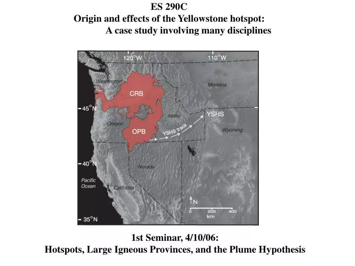
ES 290C Origin and effects of the Yellowstone hotspot: A case study involving many disciplines. 1st Seminar, 4/10/06: Hotspots, Large Igneous Provinces, and the Plume Hypothesis. J. Tuzo Wilson 1908-1003.

E N D
ES 290C Origin and effects of the Yellowstone hotspot: A case study involving many disciplines 1st Seminar, 4/10/06: Hotspots, Large Igneous Provinces, and the Plume Hypothesis
J. Tuzo Wilson 1908-1003 Throughout his career Wilson enjoyed travelling to unusual and remote places. In the mid-1930s, for example, when he was a doctoral student at Princeton University, he took time to become the first person known to have scaled Mount Hague (12,328 ft.) in Montana. When he was in Moscow in the summer of 1958 for the final meeting of the special committee which had organized the International Geophysical Year, he decided to travel to Beijing by the Trans-Siberian Railway. This led to his publication of One Chinese Moon (1959), IGY, The Year of the New Moons (1961), and Unglazed China (1973)
Hotspots - Flood Basalts - Continental Rifting Hotspots and Hawaiian Island Type Chains
Hawaiian - Emperor Seamount Chain Bend indicates change in Pacific plate movement over a hotspot(?)
W. Jason Morgan Georgia Tech, B.S. 1957 Princeton, PhD 1964 Physics *Put Wilson’s tectonics on a sphere *Ascribed hotspot tracks to plumes *Proposed plumes drive the plates *Advocated relative fixity of hotspots
Aulacogens Burke, 1977, Ann. Rev. Earth Planet. Sci. 5, 371-396 Figure 1 The sequence of swell, rift, continental rupture, and collision in aulacogen formation. A swell within a continent (top lefti is crested with volcanoes from which lavas flow and evolves into a three-rift system (upper right) with volcanoes, sediment fill (stippled), and axial dikes. Two of the rifts develop to a continental margin (lower left) and ocean (striped) forms on their sites. A miogeoclinal wedge (stippled) is deposited along the continental margin and a delta progrades down the failed rift to lie on ocean floor. Later (bottom right) another continent crosses the closing ocean and two continents collide. Rocks of the miogeoclinal wedge are thrust onto the continents and eroded by a river flowing down the aulacogen in the reversed direction. A suture zone (vertical black lines) marks th~ former site of the ocean and igneous rocks develop in the thickened continent on one side.
Aulacogens Burke, 1977, Ann. Rev. Earth Planet. Sci. 5, 371-396
To test if hotspots fixed relative to each other • Dated hotspot tracks on one plate, that have been used to derive a set of rotations describing the relative motion of the hotspot reference frame with respect to this plate. For example, for Africa we could use the dated tracks of the Walvis Ridge (from the Tristan da Cunha hotspot) and other hotspots in the South Atlantic Ocean to obtain a set of rotations describing the motion of the Africa plate with respect to the hotspots through time. • A set of rotations describing the relative motion of the hotspots with respect to another plate. For example, for the Pacific we could use the dated tracks of the Hawaiian-Emperor chain and the Louisville Ridge. • A knowledge of the past relative motions of the same two plates, derived from marine magnetic anomalies and fracture zone trends, and expressed as a set of rotations of one plate relative to another plate.
Figure 4. Gravity map of the South Atlantic [Sandwell and Smith, 1997] showing the Walvis Ridge and Rio Grande Rise hot spot system. Radiometric ages for the ridge system are shown, as listed in Table 1. Rio Grande Rise and bracketed sample number are from O’Connor and Duncan [1990]; Gough lineament data are from O’Connor and le Roex [1992]. A variety of sources concur on the age of the Parana and Etendeka volcanics [Deckart et al., 1998; Morgan, 1971; O’Connor and Duncan, 1990; Renne et al., 1996a, 1996b; Stewart et al., 1996; Wigand et al., 2004]. On the uncertainties in hot spot reconstructions and the significance of moving hot spot reference frames O’Neill, Muller, Steinberger, 2005, Geochem. Geophys. Geosyst., 6, Q04003, doi:10.1029/2004GC000784.
Figure 5. Gravity map [from Sandwell and Smith, 1997] of the St. Helena hot spot system. AC-series radiometric dates are from O’Connor and le Roex [1992]; all other dates are from O’Connor et al. [1999].
Figure 6. Gravity map [from Sandwell and Smith, 1997] of the Great Meteor hot spot system. Radiometric dates for the New England seamounts are from Duncan [1984]. An age progression from the New England seamounts to the Corner seamounts and the Great Meteor group has been shown by Tucholke and Smoot [1990] on the basis of seamount subsidence curves. Ages for White Mountains and Monteregian Hills are given by Gilbert and Foland [1986].
Figure 7. Gravity map of the Reunion hot spot system Figure 8. Gravity map of the Kerguelen hot spot system.
Fig. 13b. Predicted tracks of our fixed (brown) and moving (colored circles) hot spot reconstructions for the African plate at 10 Myr intervals. The fixed model has difficulty fitting the Ninetyeast Ridge and New England seamount chain for older times. Assumed present position of hot spots shown as blue crosses. Also shown are the predicted tracks of Muller et al. [1993] (red lines) at 10 Myr intervals for our assumed present-day positions.
Wall of Dry Falls (about 200 m high), Grand Coulee gorge, Washington, USA, in the mid-Miocene Columbia River flood basalt province, showing a section through four pahoehoe lava flow fields (1–4), each the product of a huge-volume eruption of >1000 km3 of lava. Photo by Self.
Fig. 1. Distribution of the 49 hotspots (black circles) from the catalogue used in this paper [6,11,12] superimposed on a section at (a) 500 km and (b) 2850 km depths through Ritsema et al.’s tomographic model for shear wave velocity (VS) [25]. Color code from 32% (red hues) to +2% (blue hues) velocity variation. The seven ‘primary’ hotspots outlined in this paper are shown as red circles with the first letter of their name indicated for quick reference.
Predicted Plume Uplift Uplift above a plume head, as predicted by Griffiths and Campbell (1991), compared with the uplift observed at the centre of the Emeishan flood basalt (shown in pink) by He et al. (2003). The timing and uplift shape predicted by Farnetani and Richards (1994) is similar, but they predict more uplift because they model a plume head with a higher excess temperature: 350°C as opposed to 100°C. Predicted profiles are given for maximum uplift (t = 0), when the top of the plume is at a depth of ~250 km, and 2 Myr later (t = 2 Myr), when flattening of the head is essentially complete. The uplift for the Emeishan flood basalt province is the minimum average value for the inner and intermediate zones as determined from the depth of erosion of the underlying carbonate rocks. (Campbell, 2005, Elements)
Bryce, DePaolo, Lassiter, 2005: Hawaiian plume structure, G-cubed 6 (9), 10.1029/2004GC000809 Figure 21. Schematic model of the Hawaiian plume. The central core zone of the plume is inferred to come from either the core-mantle boundary or is a tendril of a basal dense layer that is entrained by the plume along its axis. The material in the plume core is highly heterogeneous, containing materials that appear to be recycled oceanic crust as well as material that could be regarded as approximating ‘‘primitive.’’ An essential aspect of the plume core mantle is that the character of what is being melted under the volcanoes changes with time. The plume material that is just outside the plume core, which is referred to in the text as the ‘‘outer core’’ of the plume, is less heterogeneous than the plume core but still distinct from the ambient upper mantle. High 3He/4He is found only in the plume ‘‘core zone;’’ high 87Sr/86Sr is found in both the plume core and ‘‘outer core’’ zones.
Figure 1. Vertical section across three-dimensional plumes. (a) Early stage, (b) formation of a spherical head, (c) large head reaches the lithosphere, (d) 30 My after, the plume is sheared by the left moving oceanic lithosphere. (e) Early stage, (f) formation of a ‘spout’, (g) only a ‘tail’ of plume material reaches the lithosphere, (h) 30 My after.