Download
1 / 37
370 likes | 614 Views
Graphics, Tables and Basic Statistics (Chapter 3). Lecture Objectives :. Review approaches to visually displaying Data. Graphics that display key statistical features of measurements from a sample. Define the distribution of a set of data. Review common basic statistics.

E N D
Graphics, Tables and Basic Statistics (Chapter 3) Lecture Objectives : • Review approaches to visually displaying Data. • Graphics that display key statistical features of measurements from a sample. • Define the distribution of a set of data. • Review common basic statistics. • Extremes (Minimum and Maximum) • Central Tendency ( Mean, Median) • Spread (Range, Variance, Standard Deviation) • Review not so common basic statistics. • Extremes (upper and lower quartiles) • Central Tendency (Mode, Winsorized Mean) • Spread (Interquartile Range)
Graphics The visual portrayal of quantitative information • Are used to: • Display the actual data table • Display quantities derived from the data • Show what has been learned about the data from other analyses • Allow one to see what may be occurring in the data over and above what has already been described • Graphical Display • Objectives • Tabulation • Description • Illustration • Exploration “A picture is worth a thousand words…”
Objectives As you create graphics keep the following in mind. • Avoid distortion of the true story. • Induce the viewer to think about the substance, not the graph. • Reveal the data at several layers of detail. • Encourage the eye to compare different pieces. • Support the statistical and verbal descriptions of the data.
Nutrient Profiles for Selected Candy Chocolate Manufacturers Association National Confectioners Association 7900 Westpark Blvd. Suite A 320, McLean, Virginia 22102 URL: http://www.candyusa.org/nutfact.html Standard data format Qualitative characteristic Quantitative characteristics
Column chart Display the data table What are the problems with this graph?
Alternate Display Sorting and expanding the scale of the graph allows all labels to be seen as well as displaying a characteristic of the data.
Vertical Display of Data In this case, a vertical display allows better comparison of calorie amounts.
Pie Charts A pie chart is good for making relative comparisons among pieces of a whole.
Statistical Uses of Graphics • Describe Distributions of Measurements • Box & Whisker plot (Boxplot) • Histogram • Compare Distributions • Multiple Box & Whisker plots • Associations and Bivariate Distributions • Scatter plot • Symbolic scatter plot • Multidimensional Data Displays • All pairwise scatter plot • Rotating scatter plot • Graphical Methods in Support of Statistical Inference • Regression lines • Residual plots • Quantile-quantile plots • Cumulative distribution function plots • Confidence and prediction interval plots • Partial leverage plots • Smoothed curves Most of these will be demonstrated at some point in the course.
Basic Statistics • Before we get more into statistical uses of graphics, we need to define some basic statistics. These statistics are typically referred to as “descriptive statistics”, although as we will see, they are much more than that. These basic statistics address specific aspects of the distribution of the data. • What is the range of the data? • When we sort the data, what number might we see in the “middle” of the range of values? • What number tells us over what sub range do we find the bulk of the data ? We will use the calorie data to illustrate.
Extremes First, if we sort the data we can immediately identify the extremes. • Extremes • Minimum(calories) = 10 • Maximum(calories) = 210 The minimum and maximum are “statistics”. Reminder: A statistic is a function of the data. In this case, the function is very simple.
Range Range: the difference between the largest and smallest measurements of a variable. • Extremes • Minimum(calories) = 10 • Maximum(calories) = 210 Range = 210-10 = 200 Tells us something about the spread of the data. The middle of the range is a measure of the “center” of the data. Midrange = minimum + (Range/2) =10 + 200/2 =110 Is it a “good” measure of the center of the data?
Measures of Central Tendency Estimate the value that is in the center of the “distribution” of the data . Median = middle value in the sorted list of n numbers: at position (n+1)/2 = unique value at (n+1)/2 if n is an odd number or = average of the values at n/2 and n/2+1 if n is even = (160 + 160)/2 = 160 Mean = sum of all values divided by number of values (average) = (10 + 60 + 60 + 60 + … + 210 + 210)/22 = 133.6 Trimmed mean = mean of data where some fraction of the smallest and largest data values are not considered. Usually the smallest 5% and largest 5% values (rounded to nearest integer) of data are removed for this computation. = 136.0 (with 10% trimmed, 5% each tail). Again – these are statistics (functions of the data)
Let Y be the symbolic name of a random variable (e.g. a placeholder for the true name of a variable – weight, gender, time, etc.) Let yi symbolically represent the i-th value of variable Y, observed in the sample. Let the symbol, S, represent the mathematical equation for summation. Then the sample mean can be expressed as: Number of observations Symbolic “name” for sample mean Mathematical Notation We will need some mathematical notation if we are to make any progress in understanding statistics. In particular, since all statistics are functions of the data, we should be able to represent these statistics symbolically as equations using mathematical notation.
Quartiles Suppose we divide the sorted data into four equal parts. The values which separate the four parts are known as the quartiles. The first or lower quartile Q1, is the 25th percentile of the sorted data, the second quartile, Q2, is the median and the third or upper quartile, Q3, is the 75th percentile of the data. Because the sample size integer, n+1, does not always divide easily by 4, we do some estimating of these quartiles by linear interpolation between values. Here n=22, (n+1)/4=23/4=5.75, hence Q1 is three quarters between the 5th and 6th observations in the sorted list. The 5th value is 60 and the 6th value is 60, thus 60 + .75(60-60)=60. For Q2, (n+1)/2 = 23/2 = 11.5, e.g. half way between the 11th and 12th obs. Q2 = 160 + .5(160-160) = 160. For Q3, 3(n+1)/4 = 3(23)/4 = 69/4 = 17.25, e.g a quarter of the way between the 17th and 18th observations. Q3 = 180 + .25(180-180) = 180
Percentiles 100pth Percentile: that value in a sorted list of the data that has approx p100% of the measurements below it and approx (1-p)100% above it. (The p quantile.) Distribution function 0 < p < 1 Examples: Q1 = 25th percentile Q2 = 50th percentile Q3 = 75th percentile • Ott & Longnecker suggest finding a general 100pth percentile via a complicated graphical method (pp. 87-90). • We will relegate these elaborate calculations to software packages… • We will however return to this later when we discuss QQ-Plots.
Simplified Quartiles A simpler way to find Q1 & Q3 is as follows: Order the data from the lowest to the highest value, and find the median. Divide the ordered data into the lower half and the upper half, using the median as the dividing value. (Always exclude the median itself from each half.) Q1 is just the median of the lower half. Q3 is just the median of the upper half. Ex: For the candy data we still get Q1=60 and Q3=180. Ex: {3, 4, 7, 8, 9, 11, 12, 15, 18}. We get Q1=(4+7)/2=5.5 and Q3=(12+15)/2=13.5.
Measures of Variability Interquartile Range (IQR): Difference between the third quartile (Q3) and the first quartile (Q1). Quartiles: Q1 = 25th = 60 Q2 = 50th = median = 160 Q3 = 75th = 180 IQR = Q3-Q1 = 180 - 60 = 120 • Range • Interquartile Range • Variance • Standard Deviation
Variance and Standard Deviation Sample Mean Standard Deviation: The square root of the variance. Variance: The sum of squared deviations of measurements from their mean divided by n-1. Rough approximation for large n: srange/4. These measure the spread of the data.
Using Excel Data Analysis Tool Under the “Tools” menu in Excel there is a tool called “Data Analysis”. This tool is not normally loaded when the Excel default installation is used so you may have to load it yourself. This will require the Excel CD. Use the Tools > Add Ins option, select the Data Analysis tool and add it to your menu.
Excel Data Analysis Tool Select the Data Analysis Tool Select Descriptive Statistics The menu below appears. Enter the Input Range and check the output options desired.
Excel Descriptive Statistics Output You should be able to easily identify the basic statistics we have described so far. Note: the variance is not in this list. This is typical of statistics packages. Since the variance is simply the square of the Standard Deviation, it is often considered redundant. Learn to use the Excel Help files. Type “Statistic” in the Excel Help Keyword dialog for a list of helps available.
Importing a text data file in standard format into Minitab Pull down menus Session worksheet with script commands Spreadsheet like data area
Computing Descriptive Stats Descriptive Statistics Variable N Mean Median TrMean StDev SEMean calories 22 133.6 160.0 136.0 60.5 12.9 Variable Min Max Q1 Q3 calories 10.0 210.0 60.0 180.0
Frequency Table A tabular representation of a set of data. A frequency table also describes the distribution of the data and facilitates the estimation of probabilities. The “Histogram” dialog in the Excel Data Analysis Tool can be used to create this table. But it is not straightforward. Mode = most abundant
Stem and Leaf Plot Rough grouping or “binning” of the data. Histogram of calories N = 22 Midpoint Count 20 1 * 40 0 60 5 ***** 80 1 * 100 0 120 0 140 3 *** 160 6 ****** 180 2 ** 200 1 * 220 3 *** • A printer graph of the frequency table. • Easy to do by hand. • Quick visualization of the data.
Box Plot for Calories A visualization of most of the basic statistics. Maximum 75th percentile (Q3) Interquartile range Median (Q2) 25th percentile (Q1) Minimum Box Plot (SAS Proc Insight) Is there an Excel Tool? No.
Percentiles 100pth Percentile: that value in a sorted list of the data that has approx p100% of the measurements below it and approx (1-p)100% above it. (The p quantile.) Smoothed histogram 0 < p < 1 Examples: Q1 = 25th percentile Q2 = 50th percentile Q3 = 75th percentile A distribution is said to be symmetric if the distance from the median to the 100pth percentile is the same as the distance from the median to the 100(1-p)th percentile. Otherwise the distribution is said to be skewed. In the case above, the distribution is skewed to the rightsince the right tail is longer than the left tail.
Frequency Histogram 9 8 7 6 y c n 5 e u q e 4 r F 3 2 1 0 0 5 0 1 0 0 1 5 0 2 0 0 c a l o r i e s A graphical presentation of the frequency table where the relative areas of the bars are in proportion to the frequencies. This is a frequency histogram Frequency Bin width
Density Histogram A density histogram (or simply a histogram) is constructed just like a frequency histogram, but now the total area of the bars sums to one. This is accomplished by rescaling the vertical axis. Instead of frequencies, the vertical axis records the rescaled value of the density. Histograms have important ties to probability. Sum of shaded area is equal to one.
Number of Bins for Histograms Smoothed histogram or density curve. Six bins Eleven bins Five bins How we view the “distribution” of a dataset can depend on how much data we have and how it is binned.
Scatterplot Beware, changing the relative lengths of the axes can change how the relationship is perceived. Graphics to examine relationships Is the relationship linear or non-linear?
Matrix Plot View multiple variables at one time.
Three-D Views Brushing the plot to identify interesting points.
Chernoff Faces Displaying multiple variables symbolically.