
Exploring WFC3 Slitless Spectroscopy: Grism Parameters and Calibration for HST Observations
E N D
Presentation Transcript
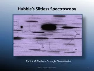
WFC3 slitless spectroscopy Harald Kuntschner Martin Kümmel, Jeremy R. Walsh (ST-ECF) WFC3-team at STScI and NASA Science with the new HST after SM4
WFC3 Grism Parameters Disperser Channel Wavelength Resolution* Å/pixel TiltX Length range (Å) (deg.) (pix) G280 UVIS 2000-4000 70@3000 Å 13 -2.8 250 G102 IR 7800-10700+ 210@10000 Å 25 +0.6 210 G141 IR 10500-17000+ 130@14000 Å 47 +0.3 130 *Resolution based on FWHM of Gaussian core in cross-dispersion direction XTilt to positive X axis +Limits at 2% transmission Science with the new HST after SM4
WFC3-IR G141Ground calibration; simulated single point source detector defects Combined white light + direct image Target position on direct image 0th order +1st order Science 1.1 -1.7mu +2nd order +3rd order 1014 pixel (full size) ~130 arcsec Science with the new HST after SM4
WFC3-IR G141 trace and dispersion calibration • Linear trace solutions (but 2-dim variations) • Linear dispersion solutions with rms < 5 Å • Dispersion: 46.9 Å/pixel (130 pixel length) • 2-dim solution varies from 45 to 48 Å/pixel dispersion * Data points omitted in fit due to wavelength shift caused by steep sensitivity decline Science with the new HST after SM4
WFC3-IR G141 Throughput • +1st order • Peak efficiency of ~40% at 1420 - 1640nm • Good sensitivity range: 1120 - 1660nm • +2nd order • Efficiency < 6% • 0th order • Efficiency < 1.5% 0th +1st +2nd +3rd Science with the new HST after SM4
WFC3-IR G102Ground calibration; simulated point source detector defects Combined white light + direct image Target position on direct image 0th order +1st order Science 0.8 - 1.1mu +2nd order 1014 pixel (full size) ~130 arcsec Science with the new HST after SM4
WFC3 G102 Trace and Dispersion • Similar to G141 linear trace and dispersion relations well reproduced by a simple 2-dim solution • Dispersion 24.6 Å/pixel (210 pixel length in +1st order) • 2-dim solution ranging from 24.0 - 25.5 Å/pixel Science with the new HST after SM4
WFC3-IR G102 Throughput • +1st order • Peak efficiency of ~30% at 960 - 1120nm • Good sensitivity range: 840 - 1140nm • +2nd order • Efficiency < 5% • 0th order • Efficiency < 1.5% 0th +1st +2nd Science with the new HST after SM4
WFC3-UV G280 Order overlap 0th +3rd 200nm Combined monochromator steps 330nm +2nd +1st 0th order +1st -1st Higher orders +2nd Higher orders -2nd 4096 pixel (full size) 160 arcsec Science with the new HST after SM4
WFC3-UV G280 • Trace: 5th order polynomial fits • Dispersion: 4th order polynomial needed to achieve good fit (rms ~ 0.2 pixel) • ~13 Å per pixel • At least +8 to -8 orders visible • Order overlap between +1st and +2nd beyond ~380nm • Heavy order overlap for > +2 orders Trace Science with the new HST after SM4
WFC3-UV G280 Throughput • 1st order • Peak efficiency of 24% at 240nm • 'Good' sensitivity range: 200 - 330nm • 2nd order • Efficiency < 2% • 0th order • Efficiency equal to first order at 330nm and rising 0th order dominates ! +2nd +1st 0th -1st -2nd Science with the new HST after SM4
Limiting magnitudes V-band detection limits for point source, 1-hour exposure and S/N=5 See Instrument Handbook See also posters by Kümmel et al. and Pirzkal et al. Science with the new HST after SM4
How to design observations? F150W and IR G141 with M51 image, galaxy images and Gaussians (for HII regions and stars) Simulated dispersed image Simulated direct image Science with the new HST after SM4
The simulation package aXeSIM • PYRAF package (ST-ECF Webpage, STSDAS in ~Jul ‘08) designed and supported at ST-ECF • One command to run full multi-object simulation – simdata • Simple object shape and spectra as built-in defaults • Produces associated direct image (opt.) • Performs default extraction of simulated spectra (opt.) • Adds noise (opt.) See poster by Kümmel et al. Science with the new HST after SM4
UV G280 - subarray, not to scale UDF simulations Direct image Dispersed image F160W < 23.0, “noise free” simulation to show 2-dim distribution Science with the new HST after SM4
Extraction software http://www.stecf.org/ • ST-ECF offers a semi-automatic extraction software (aXe) to extract fully calibrated 1-dim spectra from WFC3 grism observations; including contamination estimates • The software is already successfully being used for ACS grisms since 2003 • Available as part of STSDAS and from ST-ECF Web pages Science with the new HST after SM4
Summary • Highly efficient and well behaved IR grisms • Open up wavelength not accessible from the ground! • Challenging UV grism (order overlap, bent traces, strong 0th order…) • Software support with 2-dim simulation and data extraction packages, as well as general user support and calibration reference files available from ST-ECF (http://www.stecf.org/) • Existing, good experience with ACS grisms and NICMOS HLA project Science with the new HST after SM4