Slitless Spectroscopy with HST Instruments
150 likes | 305 Views
Slitless Spectroscopy with HST Instruments. Jeremy Walsh, Martin Kümmel & Harald Kuntschner , ST-ECF Former group contributors: Soeren Larsen, University of Utrecht Anna Pasquali , MPIA, Heidelberg Nor Pirzkal , STScI. HST slitless instrument modes - summary.

Slitless Spectroscopy with HST Instruments
E N D
Presentation Transcript
Slitless Spectroscopy with HST Instruments Jeremy Walsh, Martin Kümmel & HaraldKuntschner, ST-ECF Former group contributors: Soeren Larsen, University of Utrecht Anna Pasquali, MPIA, Heidelberg Nor Pirzkal, STScI STScI Calibration Workshop 21-23 July 2010
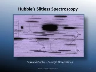
Elements of slitless spectroscopy • No slit(s) – each dispersed object forms its own ‘virtual’ slit • Effective spectral resolution depends on object ‘size’ in dispersion direction • Multiple spectral orders (grism, not prism) • Spectra can overlap → contamination • Background integrated over whole disperser passband (with gradients in dispersion direction), different from filters • Each slitless spectrum must have λ-calibration to be flat fielded WFC3 G141 WFC3 G141 median sky
Calibrations, calibrations See talk by H. Kuntschner on WFC3 NIR grism calibration • Reliance on automatic spectral extraction process imposes strong demands on calibration (initially ground, amended by in-orbit). Field variations allowed for • Position and trace of spectra from stars • Wavelength calibration (WR stars and AGN [ACS], PN [NICMOS and WFC3]) over whole field • Sensitivity from spectrophotometric standard stars (to <5%, aim 2%) • Flat field coefficient cube F(x,y,λ) - established on- ground with monochromatic flats, supplement by in-orbit filter flats for large scale illumination. Applied as polynomial fit of variation of normalised flat field v.λ • Grism (sky) background image from median combination of many grism images for global removal of background
Slitless extraction software See poster W9 by M. Kümmel on WFC3 NIR grism reduction • Simulations essential for software development and testing and as a proposal tool (esp. contamination mitigation strategies). Code derived from aXe contamination flagging • Same configuration file as aXe provides instrument specificity • Reduce simulations as real data • Employ simulated slitless images for completeness estimation, S/N determination, etc. • Instrument independent package – all instrument parameters from set of files • Configuration file specifying trace, dispersion and files: • Flat field cube • Background image • Sensitivity v. λ per order • Originally developed for ACS, then applied to NICMOS (G141) and WFC3 • HLA releases of NICMOS G141 and ACS G800L spectra • Also applied to VLT FORS2 MXU data and Euclid (simulations)
Realities of slitless spectra • Although several grism orders present, including –ve orders, no scientific exploitation other than +1st order to date • Zeroth order dispersed by the prism on which grating is ruled • On account of large angular offset, higher orders are increasingly out of focus • Multiple rolls are always helpful to ensure some uncontaminated spectra, but beware of combining spectra of extended objects at different rolls • The ‘virtual’ slit for an extended object is not along the major axis of the target (see Freudling et al. 2008, for correction) • Sensitivity established on point sources only, correction required for extended sources, otherwise 1D spectra have ‘ears’ Same target PAs differ by 122˚
Developments • Use of drizzle software (with bad pixel rejection) to combine dithered spectra • Cross correlate stellar spectra against templates to derive mean improvement to wavelength zero point per grism image (implemented in HLA ACS grism project) • What to do about contamination? Contaminating spectra based only on photometry so spectrum crude. Subtracting the contamination may not be justified. Might consider iterative approach • Slitless spectra of complex objects may look confusing; but restoration techniques bring gains. Extra information of object positions can be used to decompose point source(s) spectra from complex extended object spectra
Example is Lucy iterative decomposition of 10 strong lens knots in a field elliptical galaxy (ACS data, Blakeslee et al. 2004). Modification of IRAF task stecf.specinholucy for slitless spectra
Summary • Slitless spectroscopy with HST is very sensitive – low background from space, high spatial resolution, compact PSF, efficient grisms • Slitless spectroscopy not a ‘difficult’ technique. With care automatic extraction of thousands of spectra achievable • HLA ACS G800L archive of 47919 spectra released – reduced with fully automatic pipeline PHLAG from archive download of raw data to science ready 1D and 2D spectra (and images) • Look forward to a surge of slitless grism science from WFC3 NIR
Examples previews Low-redshift star-burst galaxy M-star 1.6” Bright elliptical at z=0.62 BAL QSO at z=2.81
Flux std star GD153 SMOV data G102 G141
Euclid (ESA Dark Energy Mission)Slitless Simulations with aXeSim ECF collaboration with Bologna, Milan, Durham (as part of NearIR Spectrograph consortium lead by A.Cimatti) End-to-end simulations of a spectroscopic slitless survey to measure DE equation of state parameters with Baryonic Acoustic Oscillations: Determination of limiting flux in Hα line and continuum Determination of redshift success rate (confusion) Determination of redshift accuracy Verify science requirements (cosmological parameters, additional science) • Drive instrument requirements/design and survey strategy • Identify critical areas (e.g. data reduction and analysis) • Assess impact on science goals of slitless vs DMD-multi-slit approach (DMD optional mode subject to technological readiness) • Results regularly reported to Euclid Study Science Team and presented in the Euclid yellow book (ESA Cosmic Vision M-class missions presentation event, Dec 1st 2009)