Download
1 / 19
190 likes | 262 Views
Lecture 16:. Univariate statistics, The Normal Curve and intro to Hypothesis Testing. Assn 2 Comments. Using Central Tendencies in Recoding. “collapsing” variables. Dispersion. Range Difference between highest value and the lowest value. Standard Deviation

E N D
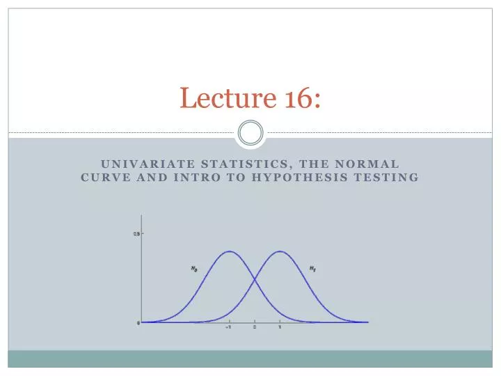
Lecture 16: Univariate statistics, The Normal Curve and intro to Hypothesis Testing
Using Central Tendencies in Recoding • “collapsing” variables
Dispersion • Range • Difference between highest value and the lowest value. • Standard Deviation • A statistic that describes how tightly the values are clustered around the mean. • Variance • A measure of how much spread a distribution has. • Computed as the average squared deviation of each value from its mean
Properties of Standard Deviation • Variance is just the square of the S.D. (or, S.D is the square root of the variance) • If a constant is added to all scores, it has no impact on S.D. • If a constant is multiplied to all scores, it will affect the dispersion (S.D. and variance) S = standard deviationX = individual scoreM = mean of all scoresn = sample size (number of scores)
Why Variance Matters… • In many ways, this is the purpose of many statistical tests: explaining the variance in a dependent variable through one or more independent variables.
Common Data Representations • Histograms (hist) • Simple graphs of the frequency of groups of scores. • Stem-and-Leaf Displays (stem) • Another way of displaying dispersion, particularly useful when you do not have large amounts of data. • Box Plots (graph box) • Yet another way of displaying dispersion. Boxes show 75th and 25th percentile range, line within box shows median, and “whiskers” show the range of values (min and max)
Issues with Normal Distributions • Skewness • Kurtosis
Estimation and Hypothesis Tests: The Normal Distribution • A key assumption for many variables (or specifically, their scores/values) is that they are normally distributed. • In large part, this is because the most common statistics (chi-square, t, F test) rest on this assumption.
Logic of Hypothesis Testing • Null Hypothesis: • H0: μ1 = μc • μ1is the intervention population mean • μc is the control population mean • In English… • “There is no significant difference between the intervention population mean and the control population mean” • Alternative Hypotheses: • H1: μ1 < μc • H1: μ1 > μc • H1: μ1 ≠ μc
Conventions in Stating Hypotheses • Three basic approaches to using variables in hypotheses: • Compare groups on an independent variable to see impact on dependent variable • Relate one or more independent variables to a dependent variable. • Describe responses to the independent, mediating, or dependent variable.
The z-score • Infinitely many normal distributions are possible, one for each combination of mean and variance– but all related to a single distribution. • Standardizing a group of scores changes the scale to one of standard deviation units. • Allows for comparisons with scores that were originally on a different scale.
z-scores (continued) • Tells us where a score is located within a distribution– specifically, how many standard deviation units the score is above or below the mean. • Properties • The mean of a set of z-scores is zero (why?) • The variance (and therefore standard deviation) of a set of z-scores is 1.
Area under the normal curve • Example, you have a variable x with mean of 500 and S.D. of 15. How common is a score of 525? • Z = 525-500/15 = 1.67 • If we look up the z-statistic of 1.67 in a z-score table, we find that the proportion of scores less than our value is .9525. • Or, a score of 525 exceeds .9525 of the population. (p < .05) • Z-score table
Sampling Distributions, N, and Expected Values • Sampling Distribution • The probability distribution of the sampling means • As ‘N’ increases, we know more about the variability of our variable of interest, and can make better judgments about the possible population mean. • Expected Values • For continuously distributed variables, the expected value is the mean.