Download
1 / 19
190 likes | 210 Views
Explore efficient methods like the Tearing and Relaxation algorithms for symbolic/numeric solving of algebraically coupled equation systems. Understand techniques to optimize structure matrix zeros and tearing variables.

E N D
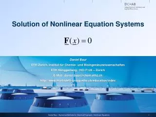
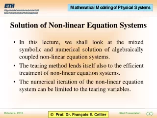
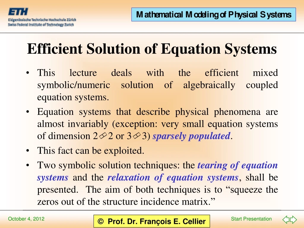
This lecture deals with the efficient mixed symbolic/numeric solution of algebraically coupled equation systems. Equation systems that describe physical phenomena are almost invariably (exception: very small equation systems of dimension 22 or 33) sparsely populated. This fact can be exploited. Two symbolic solution techniques: the tearing of equation systems and the relaxationof equation systems, shall be presented. The aim of both techniques is to “squeeze the zeros out of the structure incidence matrix.” Efficient Solution of Equation Systems
Tearing algorithm Relaxation algorithm Table of Contents
The tearing method had been demonstrated various times before. The method is explained here once more in a somewhat more formal fashion, in order to compare it to the alternate approach of the relaxation method. As mentioned earlier, the systematic determination of the minimal number of tearing variables is a problem of exponential complexity. Therefore, a set of heuristics have been designed that are capable of determining good sub-optimal solutions. The Tearing of Equation Systems I
1: u = f(t) 2: u – u1 – u2 = 0 3: u1 – L1· di1 /dt = 0 4: u2– L2 · di2 /dt = 0 5: i – i1 = 0 6: i1– i2 = 0 Constraint equation 1: u = f(t) 2: u – u1 – u2 = 0 3: u1 – L1· di1 /dt = 0 4: u2– L2 · di2 /dt = 0 5: i – i1 = 0 6: i1– i2 = 0 7: di1 /dt - di2 /dt = 0 1: u = f(t) 2: u – u1 – u2 = 0 3: u1 – L1· di1 = 0 4: u2– L2 · di2 /dt = 0 5: i – i1 = 0 6: i1– i2 = 0 7: di1 - di2 /dt = 0 Integrator to be eliminated di1 /dt Tearing of Equations: An Example I
Algebraically coupled equation system in four unknowns 1: u = f(t) 2: u – u1 – u2 = 0 3: u1 – L1· di1 = 0 4: u2– L2 · di2 /dt = 0 5: i – i1 = 0 6: i1– i2 = 0 7: di1 - di2 /dt = 0 1: u = f(t) 2: u – u1 – u2 = 0 3: u1 – L1· di1 = 0 4: u2– L2 · di2 /dt = 0 5: i – i1 = 0 6: i1– i2 = 0 7: di1 - di2 /dt = 0 Choice u1 1: u – u1 – u2 = 0 2: u1 – L1· di1 = 0 3: u2– L2 · di2 /dt = 0 4: di1 – di2 /dt = 0 1: u1= u – u2 2: di1 = u1/ L1 3: u2= L2 · di2 /dt 4: di2 /dt = di1 1: u – u1 – u2 = 0 2: u1 – L1· di1 = 0 3: u2– L2 · di2 /dt = 0 4: di1 – di2 /dt = 0 Tearing of Equations: An Example II
1: u1= u – u2 2: di1 = u1/ L1 3: u2= L2 · di2 /dt 4: di2 /dt = di1 u1= u – u2 = u –L2 ·di2 /dt = u – L2 ·di1 = u – (L2 / L1 ) ·u1 1: u = f(t) 3: u1 – L1· di1 = 0 4: u2– L2 · di2 /dt = 0 5: i – i1 = 0 6: i1– i2 = 0 7: di1 - di2 /dt = 0 L1 ·u 2: u1= [ 1 + (L2 / L1 ) ] ·u1= u L1 + L2 L1 ·u u1= L1 + L2 Tearing of Equations: An Example III
1:u = f(t) 3:di1 = u1/ L1 4:di2 /dt = di1 5:u2= L2 · di2 /dt 6:i1= i2 7: i = i1 1: u = f(t) 3: u1 – L1· di1 = 0 4: u2– L2 · di2 /dt = 0 5: i – i1 = 0 6: i1– i2 = 0 7: di1 - di2 /dt = 0 1: u = f(t) 3: u1– L1· di1 = 0 4: u2– L2 · di2 /dt = 0 5: i – i1 = 0 6: i1– i2 = 0 7: di1- di2 /dt = 0 L1 L1 L1 ·u ·u ·u 2: u1= 2: u1= 2:u1= L1 + L2 L1 + L2 L1 + L2 Question: How complex can the symbolic expressions for the tearing variables become? Tearing of Equations: An Example IV
In the process of tearing an equation system, algebraic expressions for the tearing variables are being determined. This corresponds to the symbolic application ofCramer’s Rule. A·x = bx = A-1·b (A† )ij = (-1)(i+j) · |A j,i| ; A† A-1 = |A| The Tearing of Equation Systems II
u1 u2 1 1 0 0 0 - L1 1 0 0 0 -1 - L2 1 0 0 1 u 0 0 0 di1 di2 /dt L1 . = ·u = L1 + L2 0 -1 - L2 0 0 1 - L1 1 0 u1= · u 1 1 0 0 0 - L1 1 0 0 0 -1 - L2 1 0 0 1 Tearing of Equations: An Example V
Cramer’s Rule is of polynomial complexity. However, the computational load grows with the fourth power of the size of the equation system. For this reason, the symbolic determination of an expression for the tearing variables is only meaningful for relatively small systems. In the case of bigger equation systems, the tearing method is still attractive, but the tearing variables must then be numericallydetermined. The Tearing of Equation Systems III
The relaxation method is a symbolic version of a Gauss elimination without pivoting. The method is only applicable in the case of linear equation systems. All diagonal elements of the system matrix must be 0. The number of non-vanishing matrix elements above the diagonal should be minimized. Unfortunately, the problem of minimizing the number of non-vanishing elements above the diagonal is again a problem of exponential complexity. Therefore, a set of heuristics must be found that allow to keep the number of non-vanishing matrix elements above the diagonal small, though not necessarily minimal. The Relaxation of Equation Systems I
1: u – u1 – u2 = 0 2: u1 – L1· di1 = 0 3: u2– L2 · di2 /dt = 0 4: di1 – di2 /dt = 0 u1 + u2 = u u1 - L1 · di1 = 0 di2 /dt - di1 = 0 u2- L2 · di2 /dt = 0 The non-vanishing matrix elements above the diagonal correspond conceptually to the tearing variables of the tearing method. u1 u2 1 1 0 0 0 - L1 1 0 0 0 -1 - L2 1 0 0 1 u 0 0 0 di1 di2 /dt . = Relaxing Equations: An Example I
di1 di2 /dt - L1 1 0 0 -1 - L2 c1 0 1 c2 0 0 . = u1 u2 u2 1 1 0 0 0 - L1 1 0 0 0 -1 - L2 1 0 0 1 u 0 0 0 di1 di2 /dt . = c1= -1 c2 = -u Relaxing Equations: An Example II Gauss elimination technique:
di2 /dt u2 di2 /dt u2 -1 - L2 -1 - L2 c3 1 c3 1 c4 0 c4 0 . . = = c3= c1/ L1 c4 = c2/ L1 di1 di2 /dt - L1 1 0 0 -1 - L2 c1 0 1 c2 0 0 . = u2 . = c5 u2 c6 c5= 1 - L2 · c3 c6 = - L2 · c4 Relaxing Equations: An Example III
di2 /dt u2 -1 - L2 c3 1 c4 0 . = di1 di2 /dt - L1 1 0 0 -1 - L2 c1 0 1 c2 0 0 . = u2 . = c5 u2 c6 u2= c6/c5 di1= (c2 – c1·u2) / (-L1) Relaxing Equations: An Example IV Gauss elimination technique: di2 /dt= (c4 – c3·u2) / (-1)
By now, all required equations have been found. They only need to be assembled. u1 u2 1 1 0 0 0 - L1 1 0 0 0 -1 - L2 u1 = u– u2 1 0 0 1 u 0 0 0 di1 di2 /dt . = Relaxing Equations: An Example V
1: u – u1 – u2 = 0 2: u1 – L1· di1 = 0 3: u2– L2 · di2 /dt = 0 4: di1 – di2 /dt = 0 Relaxing Equations: An Example VI u = f(t) c1 = -1 c2= -u c3 = c1 / L1 c4= c2 / L1 c5 = 1 - L2 · c3 c6= - L2 · c4 u2 = c6 / c5 di2 /dt= (c4 – c3·u2) / (-1) di1 = (c2 – c1·u2 ) / (-L1) u1= u– u2 i1= i2 i = i1 c1 = -1 c2= -u c3 = c1 / L1 c4= c2 / L1 c5 = 1 - L2 · c3 c6= - L2 · c4 u2 = c6 / c5 di2 /dt= (c4 – c3·u2) / (-1) di1 = (c2 – c1·u2 ) / (-L1) u1= u– u2
The relaxation method can be applied symbolically to systems of slightly larger size than the tearing method, because the computational load grows more slowly. For some classes of applications, the relaxation method generates very elegant solutions. However, the relaxation method can only be applied to linear systems, and in connection with the numericalNewton iteration,the tearing algorithm is usually preferred. The Relaxation of Equation Systems II
Elmqvist H. and M. Otter (1994), “Methods for tearing systems of equations in object-oriented modeling,” Proc. European Simulation Multiconference, Barcelona, Spain, pp. 326-332. Otter M., H. Elmqvist, and F.E. Cellier (1996), “Relaxing: A symbolic sparse matrix method exploiting the model structure in generating efficient simulation code,” Proc. Symp. Modelling, Analysis, and Simulation, CESA'96, IMACS MultiConference on Computational Engineering in Systems Applications, Lille, France, vol.1, pp.1-12. References