Solution of Nonlinear Equation Systems
230 likes | 542 Views
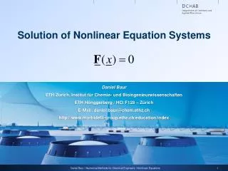
Solution of Nonlinear Equation Systems. Daniel Baur ETH Zurich, Institut für Chemie- und Bioingenieurwissenschaften ETH Hönggerberg / HCI F128 – Zürich E-Mail: daniel.baur@chem.ethz.ch http://www.morbidelli-group.ethz.ch/education/index . Zero of Nonlinear Equation Systems. Problem definition :

Solution of Nonlinear Equation Systems
E N D
Presentation Transcript
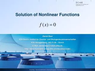
Solution of Nonlinear Equation Systems Daniel BaurETH Zurich, Institut für Chemie- und BioingenieurwissenschaftenETH Hönggerberg / HCI F128 – ZürichE-Mail: daniel.baur@chem.ethz.chhttp://www.morbidelli-group.ethz.ch/education/index Daniel Baur / Numerical Methods for Chemical Engineers / Nonlinear Equations
Zero of Nonlinear Equation Systems • Problem definition: • Find the solution of F(x) = 0, where both F and x are vector (or matrix) valued; Look for the solution either • In an interval xlb < x < xub • Or in the uncertainty interval [a, b] • Types of algorithm available: • Substitution algorithms • Methods based on function approximation • Assumptions: • At least one zero exists in the defined interval • We are looking for one zero, not all of them Daniel Baur / Numerical Methods for Chemical Engineers / Nonlinear Equations
Example • Consider the following function Daniel Baur / Numerical Methods for Chemical Engineers / Nonlinear Equations
Projection on the xy-Plane f(x,y) = 0 Daniel Baur / Numerical Methods for Chemical Engineers / Nonlinear Equations
Function Linearization • Let us again consider Taylor expansion • In matrix form, this reads • Which is equivalent to • Newton Method! Daniel Baur / Numerical Methods for Chemical Engineers / Nonlinear Equations
The Multidimensional Newton-Algorithm • Define a starting point x • Compute –F(x) • Compute J(x) • Either analytically or numerically • Solve the linear system of equations J(x)*Δx = -F(x)for Δx, then set x = x + Δx • Iterate 2 through 4 until one of the following is fulfilled • norm(F(x)) < tol(1); • norm(Δx) < tol(2); • niter > tol(3); Daniel Baur / Numerical Methods for Chemical Engineers / Numerical Quadrature
Improvements on the Algorithm • It might not be necessary to compute the Jacobian at every iteration, the algorithm can also work nicely if the Jacobian is only computed every few iterations • When doing this, instead of solving the linear system of equations, it might be more efficient to compute inv(J) when recomputing J, or factorize it in a convenient manner • A numerical Jacobian can actually lead to better results than an analytical one • Another option is to adapt the step size, so before accepting a Δx, one checks if norm(F(x+Δx)) is in fact smaller than norm(F(x)), and if not, a step of size λ*Δx with λ<1 is tried instead Daniel Baur / Numerical Methods for Chemical Engineers / Numerical Quadrature
Graphical Interpretation • Consider our example system and its linearization • If we start at (0, 0), we get two tangent planes Daniel Baur / Numerical Methods for Chemical Engineers / Nonlinear Equations
Projection on the xy-Plane Daniel Baur / Numerical Methods for Chemical Engineers / Nonlinear Equations
Effect of Different Starting Points Daniel Baur / Numerical Methods for Chemical Engineers / Nonlinear Equations
How does Matlab do it? Nonlinear Systems • fsolveis the general solver for non-linear equation systems; It can use different algorithms, namely • Trust-region algorithms: Instead of just going in the direction that the Newton step suggests, a check is performed if xk+1 is really better than xk. This is done by approximating the behavior of the function around xk (the trust-region). An optimization is then performed to find an optimal step. • Trust-region-dogleg: The so-called dogleg method is used to solve the optimization problem, which constructs the step as a convex combination of the Cauchy step (steepest descent) and a Gauss-Newton step. • Trust-region-reflective: The optimization problem is solved via a conjugate gradient method in a 2-D subspace. • The Levenberg-Marquardt method, which finds the step by solving Daniel Baur / Numerical Methods for Chemical Engineers / Nonlinear Equations
Matlab Syntax Hints • fsolveuses the syntax • x = fsolve(@nl_fun, x0, options); • where nl_fun is a function taking as input x, returning as output the function values f at x, both can be vectors or matrices • x0 is an initial guess • options can be set by options = optimset(...)to choose algorithms, give analytical Jacobians, etc.; see doc fsolve for details Daniel Baur / Numerical Methods for Chemical Engineers / Nonlinear Equations
Exercise: CSTR Multiple Steady States • Consider a CSTR where a reaction takes place • We assume the following • V = const., i.e. Qin = Qout = const. • Perfect coolant behavior, i.e. TC,in = TC,out = const. • Constant density and heat capacity of the reaction mixture • Constant reaction enthalpy • Constant feed, i.e. cA,in = const., Tin = const. Daniel Baur / Numerical Methods for Chemical Engineers / Nonlinear Equations
CSTR Mass and Energy Balances • The mass and energy balances read • With the T-dependent reaction rate constant Daniel Baur / Numerical Methods for Chemical Engineers / Nonlinear Equations
Dimensionless Mass and Energy Balances • If we define • We get a dimensionless form Daniel Baur / Numerical Methods for Chemical Engineers / Nonlinear Equations
Dimensionless CSTR Steady State • The steady state of the CSTR reads: • where uASS, uBSS and θSS are unknown Daniel Baur / Numerical Methods for Chemical Engineers / Numerical Quadrature
Dimensionless CSTR Jacobian • The Jacobian matrix of the CSTR readswhereand Daniel Baur / Numerical Methods for Chemical Engineers / Nonlinear Equations
Assignment • Implement the basic Newton method as shown on slide 6. • Use a function of the formfunction [x, info] = NewtonMethod(f, J, x0, tol);where f is a function handle to the function you want to solve, J is a function handle that returns the Jacobian matrix, x0 is an initial guess and tol is a vector of tolerances. • Use left division «\» to solve the linear system at every iteration. • Let info be a struct you can use to return additional information, like reason of termination and number of steps needed. • Use your Newton algorithm to solve the steady state CSTR numerically. Try different, reasonable starting guesses. Can you reproduce the three steady state temperatures we have found for the 1D case in the last exercise (0.96, 1.04 and 1.13)? What is the conversion? • Use α = 49.46; κ0 = 2.17e20; KC = 0.83; η = 0.33 and θC = 0.9. Daniel Baur / Numerical Methods for Chemical Engineers / Numerical Quadrature
Assignment (Continued) • Find online the function jacobianest. It is part of a user-made toolbox for estimating derivatives numerically, the DERIVESTsuite which can be found on the MatlabCentral. • Modify your Newton algorithm so that it uses jacobianest to approximate the Jacobian if the input J is empty (use isempty(J) to check). To provide an empty input, use [ ] in the call. • How many steps are required with the analytical Jacobian compared to the numerical Jacobian? Which algorithm takes longer? • What happens to the two algorithms if you use a large starting guess for theta, for example 5? Do you have an idea why this happens? Daniel Baur / Numerical Methods for Chemical Engineers / Nonlinear Equations
