Conductance Model
Conductance Model. Laurence Benjamin. Over View. Historical Development of the model Growth and the environment Competition in even-aged monocultures Competition in mixed-aged mixed species Spatial patterns Validation. Historical Development.


Conductance Model
E N D
Presentation Transcript
Conductance Model Laurence Benjamin
Over View • Historical Development of the model • Growth and the environment • Competition in even-aged monocultures • Competition in mixed-aged mixed species • Spatial patterns • Validation
Historical Development • Attempts to model the effect density and time for growth of horticultural crops (Scaife, Cox and Morris, 1987) • Assumed that growth is driven by temperature, but also modified by light into a single effective day degree (EDD). • Used an reciprocal equation
Effective Day Degrees (EDD) T is temperature, Tb is the base temperature, I is radiant energy. q is a term which is a weighting factor for the relative importance of the temperature and light for growth.
The Reciprocal Equation Used in many areas • Combined effects on growth of two mineral nutrients (Balmukand, 1928) • Combined effect of several resistances in parallel in an electrical circuit (Ohm’s Law) • To calculate the focal length of a lens (or concave/convex mirror) given the distance from the lens from the object and image
Further Development • Emphasis on combining effects of all environmental factors – not just a modification of day degrees (Aikman and Scaife, 1993) • C is CO2 concentration, and Γ* is the compensation concentration • The are terms a, b and c are called conductances
Plant Environment Time (PET) • Each unit of chronological time, u, can accumulate any amount of ‘plant environment time’
The Expolinear Model and PET • The growth rate of plants is the product of mass, m, and the fraction of light intercepted, f
The Expolinear Model and PET • The fraction of intercepted light is given by where L is the leaf area index and k is the extinction coefficient for light
The Expolinear Model and PET Aikman and Scaife derived the follow equation to predict plant weight, w where F is the leaf area ratio, f0is the value of f at the start of crop growth and n is plant density
A New Model A weakness was that the self-shading function restricts all environmental parameters. Aikman and Scaife proposed:- where φ is the efficiency of light interception per unit leaf area
The Self-Shading Function The self-shading function was defined as whereslis the leaf area per plant, where
PET and New Model An important distinction in the new model introduced by Aikman and Scaife is that there is no longer a common PET for all plants, but PET is affected by density and plant weight
Modelling Individual Plant Growth • Light is intercepted only within the the crown zone area of individual plants • Aikman and Watkinson (1980) proposed that Where sz is the crown zone area and A is an allometric constant
Light Interception for Individual Plants The LAI within a shoot crown, Lz, is given by The fraction of light, fz, intercepted in the crown zone is given by
Growth Rate for Individual Plants If light is the only limiting factor, growth rate, dw/dt, at time t is:- Which is:- α is the conversion of light to dry matter
Interactions Between Plants If there are n plants per unit area, when crown zone areas of adjacent plants meet then
Dynamics in Even-Aged Communities • Initially all plants grow as though isolated. • When the sum of crown zone areas match the ground area, then canopy closure commences
LAI and Plant Size • An important consequence of this eqn is that the within crown zone LAI is greater for larger plants. • The numerator is proportional to w, but the denominator is proportional to w2/3
Processes During Canopy Closure • The larger plants (with greater within-crown LAI) will continue to grow as though isolated, but the smaller plants will occupy only the remaining space. • If there are two cohorts of density n1and n2, then the crown zone area of each cohort 2 plant is:-
The Community During Canopy Closure • The ‘squeezing’ of the smaller plants will continue until the within-crown zone area of large and small plants are matched. • During canopy closure, asymmetric competition for light occurs • growth rates diverge • Plant-to-plant variability increases
Canopy Closure Completion • During canopy closure an ‘underclass’ of squeezed plants and an upper class of plants growing as though isolated exist. • As canopy closure proceeds more plants fall into the under class • Eventually all plants are in the under class and canopy closure is completed
Canopy Closure • After canopy closure all plants grow as in proportion to their leaf area • Plants grow in proportion to their weight • Variability (Coefficient of Variation) remains constant.
Uneven Plant Heights • The plants will form different storeys • Within each storey the process of canopy closure is as for the even height communities • The plant density within each storey is lower than that for the entire community • The light available for growth is that not intercepted by upper storeys
Competition Between Plants of different Species • The algorithms to describe competition between plants is not dependent on the species • By using parameter values of the species, it is possible to simulate inter-species competition without the need to determine interaction terms
Spatial Pattern • Benjamin (1999) for monocrops assumed that the crown zone areas could overlap, and that the crop growth rate in the region, i, of overlap would be determined by
Spatial Pattern • The crop growth at that location could then be partitioned between all the plants in proportion to their ‘encounters’. • ‘Encounters’ were based on either:- • the number of overlapping plants • the leaf area index of overlapping plants • the degree of overlap, e, experienced by the plants
Spatial Pattern • The best agreement with data was based on degree of overlap • For plants x and y with crown zone radii of R and distance apart d
Model Validation EDD and PET From weight – density relations for (Scaife et al., 1987) • cauliflower (Brassica oleracea var Botrytis L) • celery (Apium graveolens L) • leek (Allium porrum L) • lettuce (Latuca sativa L). Brewster and Sutherland (1993) • 8 Vegetable and 2 bedding plant species Tei et al. (1996) • Onion • Red Beet
dry weight (g) 1000 100 10 1 0.1 150 200 250 300 day of year Growth of Isolated Cabbage Plants
Model Validation Crown Zone Area (Aikman and Benjamin 1994) • lettuce • Onion • Red Beet
Model Validation Mixed Species Competition (Benjamin and Aikman 1995) • Carrot • Cabbage
Model Validation Allometric Relations (Park et al 2001) • Carrot • Cabbage • Clover (Trifolium repens L), • Mayweed (Matricaria inodora L) • Black nightshade (Solanum nigrum L) • chickweed (Stellaria media L) • speedwell (Veronica persica L).
10 1 0.1 0.01 0.001 0.0001 0.1 1 10 100 1000 plant dry weight (g) Plant Weight - Leaf Area and Zone Area Relations in Cabbage 1 0.1 0.01 0.001 0.1 1 10 100 1000 plant dry weight (g)
Model Validation Allometric Relations (Park et al 2001)
Model Validation Predicting Mixed Species Growth (Benjamin and Aikman, 1994) • Cabbage and Black Nightshade (Park et al 2001) • Cabbage and Speedwell
Plant dry weight (g) Days after first harvest Observed and Predicted Growth of Cabbage and Nightshade 16 observed predicted 14 cabbage nightshade 12 10 8 6 4 2 0 0 10 20 30 40
Model Validation Spatial Pattern (Benjamin 1999) • Carrots (rings of plants around focal plant and on a grid)
Conclusion Strengths • Simple • Mechanistically-based • Proven application to mixed species cropping • Potential for further development Weaknesses (opportunities for improvement) • Too simple for complex processes • Leaf deaf • Water relations • Mineral nutrients • Low temperatures • Comparison with other models Benjamin L. R . and Park S. E. (2007). The Conductance model of plant growth and competition in monocrop and species mixtures: a review. Weed Research47 284-298.