
Iterative Program Analysis
E N D
Presentation Transcript
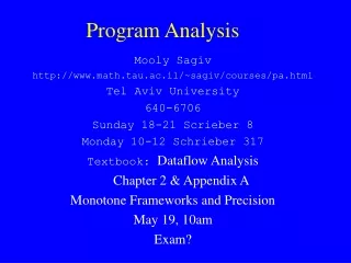
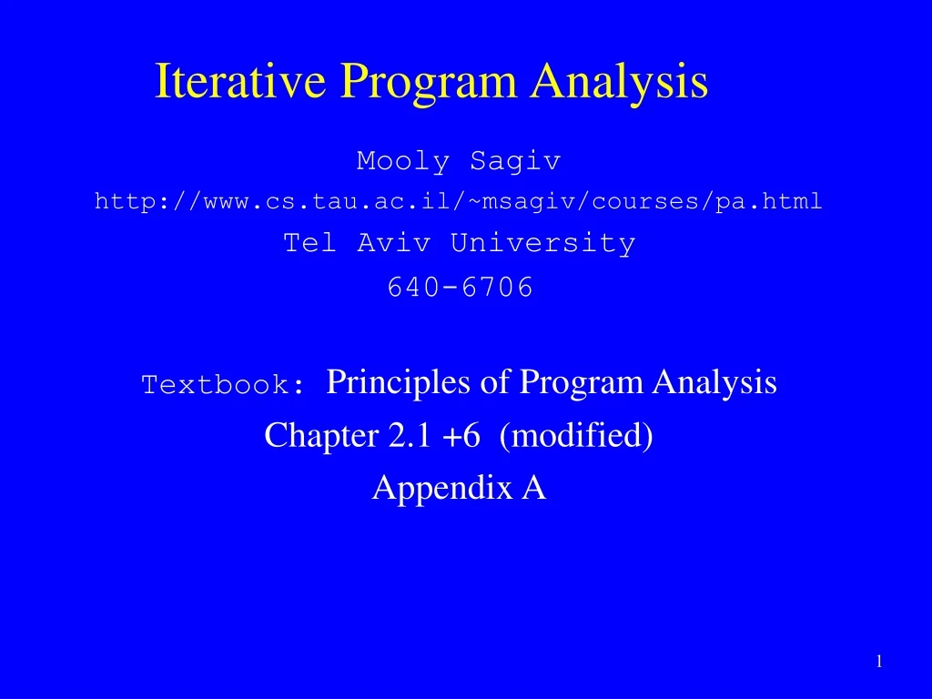
Iterative Program Analysis Mooly Sagiv http://www.cs.tau.ac.il/~msagiv/courses/pa.html Tel Aviv University 640-6706 Textbook: Principles of Program Analysis Chapter 2.1 +6 (modified) Appendix A
Outline • A gentle introduction constant propagation • Mathematical background • Chaotic iterations • Abstract interpretation • More examples • Kill/Gen Problems • Garbage variables • Pointer analysis • Stack • Heap (later)
[x0, y0, z0] [x1, y0, z3] [x1, y0, z3] [x1, y7, z3] [x0, y0, z3] [x1, y7, z3] [x3, y7, z3] [x3, y7, z3] A Simple Example Program z = 3 x = 1 while (x > 0) ( if (x = 1) then y = 7 else y = z + 4 x = 3 print y )
[x0, y0, z0] [x1, y0, z3] [x, y0, z3] [x1, y7, z3] [x1, y7, z3] [x0, y0, z3] [x3, y7, z3] [x3, y7, z3] A Simple Example Program z = 3 x = 1 while (x > 0) ( if (x = 1) then y = 7 else y = z + 4 x = 3 print y )
[x0, y0, z0] [x1, y0, z3] [x, y0, z3] [x, y7, z3] [x1, y7, z3] [x0, y0, z3] [x3, y7, z3] [x3, y7, z3] A Simple Example Program z = 3 x = 1 while (x > 0) ( if (x = 1) then y = 7 else y = z + 4 x = 3 print y )
[x0, y0, z0] [x1, y0, z3] [x, y0, z3] [x, y7, z3] [x, y7,z3] [x0, y0, z3] [x1, y7,z3] [x3, y7, z3] [x3, y7, z3] A Simple Example Program z = 3 x = 1 while (x > 0) ( if (x = 1) then y = 7 else y =z + 4 x = 3 print y )
[x0, y0, z0] [x1, y0, z3] [x, y0, z3] [x1, y7, z3] [x, y7,z3] [x0, y0, z3] [x1, y7,z3] [x, y7,z3] [x3, y7, z3] [x3, y7, z3] A Simple Example Program z = 3 x = 1 while (x > 0) ( if (x = 1) then y = 7 else y =z + 4 x = 3 print y )
[x0, y0, z0] [x1, y0, z3] [x, y0, z3] [x1, y7, z3] [x0, y0, z3] [x, y7,z3] [x, y7,z3] [x3, y7, z3] [x3, y7, z3] A Simple Example Program z = 3 x = 1 while (x > 0) ( if (x = 1) then y = 7 else y =z + 4 x = 3 print y )
Computing Constants • Construct a control flow graph (CFG) • Associate transfer functions with control flow graph edges • Iterate until a solution is found • The solution is unique • But order of evaluation may affect the number of iterations
Constructing CFG z =3 z = 3 x = 1 while (x > 0) ( if (x = 1) then y = 7 else y =z + 4 x = 3 print y ) x =1 while (x>0) if (x=1) y =7 y =z+4 x=3 print y
Associating Transfer Functions z =3 e.e[z3] x =1 e.e[x1] e. if x 0 then e else while (x>0) e. if x >0 then e else if (x=1) e. if x 0 then e else e. e [x1, y , z] y =7 y =z+4 e.e e.e[y7] e.e[ye(z)+4] x=3 e.e[x3] print y
Iterative Computation [x0, y0, z0] z =3 e.e[z3] x =1 e.e[x1] e. if x 0 then e else while (x>0) e. if x >0 then e else if (x=1) e. if x 0 then e else e. e [x1, y , z] y =7 y =z+4 e.e e.e[y7] e.e[ye(z)+4] x=3 e.e[x3] print y
Iterative Computation [x0, y0, z0] z =3 e.e[z3] [x1, y0, z0] x =1 e.e[x1] e. if x 0 then e else while (x>0) e. if x >0 then e else if (x=1) e. if x 0 then e else e. e [x1, y , z] y =7 y =z+4 e.e e.e[y7] e.e[ye(z)+4] x=3 e.e[x3] print y
Iterative Computation [x0, y0, z0] z =3 e.e[z3] [x0, y0, z3] x =1 e.e[x1] e. if x 0 then e else while (x>0) e. if x >0 then e else if (x=1) e. if x 0 then e else e. e [x1, y , z] y =7 y =z+4 e.e e.e[y7] e.e[ye(z)+4] x=3 e.e[x3] print y
Iterative Computation [x0, y0, z0] z =3 e.e[z3] [x0, y0, z3] x =1 e.e[x1] e. if x 0 then e else [x1, y0, z3] while (x>0) e. if x >0 then e else if (x=1) e. if x 0 then e else e. e [x1, y , z] y =7 y =z+4 e.e e.e[y7] e.e[ye(z)+4] x=3 e.e[x3] print y
Iterative Computation [x0, y0, z0] z =3 e.e[z3] [x0, y0, z3] x =1 e.e[x1] e. if x 0 then e else [x1, y0, z3] while (x>0) e. if x >0 then e else [x1, y0, z3] if (x=1) e. if x 0 then e else e. e [x1, y , z] y =7 y =z+4 e.e e.e[y7] e.e[ye(z)+4] x=3 e.e[x3] print y
Iterative Computation [x0, y0, z0] z =3 e.e[z3] [x0, y0, z3] x =1 e.e[x1] e. if x 0 then e else [x1, y0, z3] while (x>0) e. if x >0 then e else [x1, y0, z3] if (x=1) e. if x 0 then e else e. e [x1, y , z] y =7 y =z+4 [x1, y0, z3] e.e e.e[y7] e.e[ye(z)+4] x=3 e.e[x3] print y
Iterative Computation [x0, y0, z0] z =3 e.e[z3] [x0, y0, z3] x =1 e.e[x1] e. if x 0 then e else [x1, y0, z3] while (x>0) e. if x >0 then e else [x1, y0, z3] if (x=1) e. if x 0 then e else e. e [x1, y , z] y =7 y =z+4 [x1, y0, z3] e.e e.e[y7] e.e[ye(z)+4] [x1, y7, z3] x=3 e.e[x3] print y
Iterative Computation [x0, y0, z0] z =3 e.e[z3] [x0, y0, z3] x =1 e.e[x1] e. if x 0 then e else [x1, y0, z3] while (x>0) e. if x >0 then e else [x1, y0, z3] if (x=1) e. if x 0 then e else e. e [x1, y , z] y =7 y =z+4 [x1, y0, z3] e.e e.e[y7] e.e[ye(z)+4] [x1, y7, z3] x=3 e.e[x3] [x3, y7, z3] print y
Iterative Computation [x0, y0, z0] z =3 e.e[z3] [x0, y0, z3] x =1 e.e[x1] e. if x 0 then e else [x, y0, z3] while (x>0) e. if x >0 then e else [x1, y0, z3] if (x=1) e. if x 0 then e else e. e [x1, y , z] y =7 y =z+4 [x1, y0, z3] e.e e.e[y7] e.e[ye(z)+4] [x1, y7, z3] x=3 e.e[x3] [x3, y7, z3] print y
Iterative Computation [x0, y0, z0] z =3 e.e[z3] [x0, y0, z3] x =1 e.e[x1] e. if x 0 then e else [x, y0, z3] while (x>0) e. if x >0 then e else [x, y0, z3] if (x=1) e. if x 0 then e else e. e [x1, y , z] y =7 y =z+4 [x1, y0, z3] e.e e.e[y7] e.e[ye(z)+4] [x1, y7, z3] x=3 e.e[x3] [x3, y7, z3] print y
Iterative Computation [x0, y0, z0] z =3 e.e[z3] [x0, y0, z3] x =1 e.e[x1] e. if x 0 then e else [x, y0, z3] while (x>0) e. if x >0 then e else [x, y0, z3] if (x=1) e. if x 0 then e else e. e [x1, y , z] y =7 y =z+4 [x, y0, z3] e.e e.e[y7] e.e[ye(z)+4] [x1, y7, z3] x=3 e.e[x3] [x3, y7, z3] print y
Iterative Computation [x0, y0, z0] z =3 e.e[z3] [x0, y0, z3] x =1 e.e[x1] e. if x 0 then e else [x, y0, z3] while (x>0) e. if x >0 then e else [x, y0, z3] if (x=1) e. if x 0 then e else e. e [x1, y , z] [x, y0, z3] y =7 y =z+4 [x, y0, z3] e.e e.e[y7] e.e[ye(z)+4] [x1, y7, z3] x=3 e.e[x3] [x3, y7, z3] print y
Iterative Computation [x0, y0, z0] z =3 e.e[z3] [x0, y0, z3] x =1 e.e[x1] e. if x 0 then e else [x, y0, z3] while (x>0) e. if x >0 then e else [x, y0, z3] if (x=1) e. if x 0 then e else e. e [x1, y , z] [x, y0, z3] y =7 y =z+4 [x1, y0, z3] e.e e.e[y7] e.e[ye(z)+4] [x, y7, z3] x=3 e.e[x3] [x3, y7, z3] print y
Order of evaluation • The solution is unique • Different orders may converge faster • Example order: Depth First Order
Mathematical Background • Declaratively define • The result of the analysis • The exact solution • Allow comparison • Prove that the algorithm is sound by proving that the handling of atomic statements is sound
Posets • A partial ordering is a binary relation : L L {false, true} • For all l L : l l (Reflexive) • For all l1, l2, l3 L : l1 l2, l2 l3 l1 l3 (Transitive) • For all l1, l2 L : l1 l2, l2 l1 l1 = l2 (Anti-Symmetric) • Denoted by (L, ) • In program analysis • l1 l2 l1 is more precise than ll1 represents fewer concrete states than l2
Example Posets • Total orders (N, ) • Powersets (P(S), ) • Powersets (P(S), ) • Constant propagation
Posets • More notations • l1 l2 l2 l1 • l1 l2 l1 l2 l1 l2 • l1 l2 l2 l1
Upper and Lower Bounds • Consider a poset (L, ) • A subset L’ L has a lower boundl L if for all l’ L’ : l l’ • A subset L’ L has an upper boundu L if for all l’ L’ : l’ u • A greatest lower bound of a subset L’ L is a lower bound l0 L such that l l0 for any lower bound l of L’ • A lowest upper bound of a subset L’ L is an upper bound u0 L such that u0 u for any upper bound u of L’ • For every subset L’ L: • The greatest lower bound of L’ is unique if at all exists • L’ (meet) a b = {a, b} • The lowest upper bound of L’ is unique if at all exists • L’ (join) ab = {a, b}
Complete Lattices • A poset (L, ) is a complete lattice if every subset has least and upper bounds • L = (L, ) = (L, , , , , ) • = = L • = L = • Examples • Total orders (N, ) • Powersets (P(S), ) • Powersets (P(S), ) • Constant propagation
Complete Lattices • Lemma For every poset (L, ) the following conditions are equivalent • L is a complete lattice • Every subset of L has a least upper bound • Every subset of L has a greatest lower bound
Cartesian Products • A complete lattice (L1, 1) = (L1, , 1, 1, 1, 1) • A complete lattice (L2, 2) = (, , 2, 2, 2, 2) • Define a Poset L = (L1 L2 ,) where • (x1, x2) (y1, y2) if • x1 y1 and • x2 y2 • L is a complete lattice
Finite Maps • A complete lattice (L1, 1) = (L1, , 1, 1, 1, 1) • A finite set V • Define a Poset L = (VL1 ,) where • e1 e2 if for all v V • e1v e2v • L is a complete lattice
Chains • A subset Y L in a poset (L, ) is a chain if every two elements in Y are ordered • For all l1, l2 Y: l1 l2 or l2 l1 • An ascending chain is a sequence of values • l1 l2 l3 … • A strictly ascending chain is a sequence of values • l1 l2 l3… • A descending chain is a sequence of values • l1 l2 l3 … • A strictly descending chain is a sequence of values • l1 l2 l3 … • L has a finite height if every chain in L is finite • Lemma A poset (L, ) has finite height if and only if every strictly decreasing and strictly increasing chains are finite
Monotone Functions • A poset (L, ) • A function f: L L is monotoneif for every l1, l2 L: • l1 l2 f(l1 ) f(l2)
Lemma 1 Consider a lattice L. f: L L is monotone iff for all X L: {f(z) | z X } f({z | z X })
Distributive (additive functions) Consider a lattice L. f: L L is distributive if for all X L: {f(z) | z X } = f({z | z X })
f() f2() Fix(f) Red(f) f2() Ext(f) f() Fixed Points • A monotone function f: L L where (L, , , , , ) is a complete lattice • Fix(f) = { l: l L, f(l) = l} • Red(f) = {l: l L, f(l) l} • Ext(f) = {l: l L, l f(l)} • l1 l2 f(l1 ) f(l2) • Tarski’s Theorem 1955: if f is monotone then: • lfp(f) = Fix(f) = Red(f) Fix(f) • gfp(f) = Fix(f) = Ext(f) Fix(f) gfp(f) lfp(f)
Computing lfp(f) x = while f(x)x do x = f(x)
Chaotic Iterations • A lattice L = (L, , , , , ) with finite strictly increasing chains • Ln = L L … L • A monotone function f: LnLn • Compute lfp(f) • The simultaneous least fixed of the system {x[i] = fi(x) : 1 i n } for i :=1 to n do x[i] = WL = {1, 2, …, n} while (WL ) do select and remove an element i WL new := fi(x) if (new x[i]) then x[i] := new; Add all the indexes that directly depends on i to WL x := (, , …, ) while (f(x) x ) do x := f(x)
Specialized Chaotic Iterations Chaotic(G(V, E): Graph, s: Node, L: Lattice, : L, f: E (L L) ){ for each v in V to n do dfentry[v] := df[v] = WL = {1, 2, … n} while (WL ) do select and remove an element u WL for each v, such that. (u, v) E do temp = f(e)(dfentry[u]) new := dfentry(v) temp if (new dfentry[v]) then dfentry[v] := new; WL := WL {v}
[x0, y0, z0] 1 z =3 e.e[z3] 2 x =1 e.e[x1] e. if x 0 then e else 3 while (x>0) e. if x >0 then e else 4 if (x=1) e. if x 0 then e else e. e [x1, y , z] 5 6 y =7 y =z+4 e.e e.e[y7] e.e[ye(z)+4] 7 x=3 e.e[x3] 8 print y
Specialized Chaotic IterationsSystem of Equations S = dfentry[s] = dfentry[v] = {f(u, v) (dfentry[u]) | (u, v) E } FS:LnLn FS(X)[s] = FS(X)[v]= {f(u, v)(X[u]) | (u, v) E } lfp(S) = lfp(FS)
Complexity of Chaotic Iterations • Parameters: • n the number of CFG nodes • k is the maximum outdegree of edges • A lattice of height h • c is the maximum cost of • applying f(e) • • L comparisons • ComplexityO(n * h * c * k)
Soundness • Every detected constant is indeed such • Every error will be detected • The least fixed points represents all occurring runtime states
Completeness • Every constant is indeed detected as such • Every detected error is real • Every state represented by the least fixed is reachable for some input
The Abstract Interpretation Technique • The foundation of program analysis • Goals • Establish soundness of (find faults in) a given program analysis algorithm • Design new program analysis algorithms • The main ideas: • Relate each step in the algorithm to a step in a structural operational semantics • Establish global correctness using a general theorem • Not limited to a particular form of analysis
Galois Connections • Lattices Cand A and functions : C A and : AC • The pair of functions (, ) form Galois connectionif • and are monotone • a A • ( (a)) a • c C • c ((C)) • Alternatively if: c C a A (c) a iff c (a) • and uniquely determine each other
Abstract Descriptors of sets of stores Galois Connections Concrete Sets of stores