Historical Data Analysis
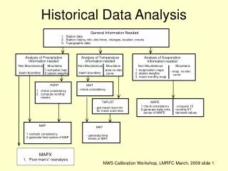
General Information Needed. 1. Station data. 2. Station history info: obs times, changes, location, moves. 3. Topographic data. Analysis of Precipitation. Analysis of Temperature. Analysis of Evaporation. Information needed. Information needed. Information needed. Non Mountainous.

Historical Data Analysis
E N D
Presentation Transcript
General Information Needed 1. Station data 2. Station history info: obs times, changes, location, moves 3. Topographic data Analysis of Precipitation Analysis of Temperature Analysis of Evaporation Information needed Information needed Information needed Non Mountainous Mountains Non Mountainous Mountains Non Mountainous Mountains 1 isohyetal map - area vs elev. 1 evaporation maps - evap. vs elev. -basin boundary -basin boundary 2 station weights curve 2 station weights curve 3 mean monthly evap . PXPP MAT - check consistency 1 check consistency 2 compute monthly means TAPLOT MAPE 1 check consistency -compute 12 - get mean max/min 2 generate daily time monthly ET for mean zone elev . series of MAPE demand values MAP MAT 1 recheck consistency - generate time 2 generate time series of MAP series of MAT. Historical Data Analysis MAPX 1. ‘Poor man’s” reanalysis
Analysis of Precipitation • Non-Mountainous Areas • Long Term Means Vary Slightly Across the Region • Station Weights Based Totally on Location • Mountainous Areas • Long Term Means Vary Across the Region • Ratio of Monthly Normals Used when Estimating Missing Data • Long Term Areal Mean Based on Isohyetal Analysis • Station Weights Typically Don’t Sum to 1.0
Analysis of Precipitation Criteria for Mountainous vs Non-MountainousArea Analysis • Mountainous Areas: any area where the long-term mean precipitation varies significantly over the area such that mean areal values cannot be computed as a weighted average based solely on the geographical location of the stations.
Analysis of PrecipitationStation Selection • Be conservative • All stations within basin • A few outside the basin for coverage and estimation of missing data • At least 5, preferably 10 years of data • Complete as possible record • Hourly stations for time disaggregation of daily stations • Go further out for mtn. areas to represent higher elevations.
Selection of Potential Precipitation Stations in Non-Mountainous Areas H H D D D D H D D D D D H D H D H D
Selection of Potential Precipitation Stations in Non-Mountainous Areas Hourly station needed to distribute nearby daily station values H H D D D D H Daily station used as estimator for nearby daily station D D D D D H D H D H D
Precipitation data Main river channel Standard Rain Gauge Boundary of drainage area
Data Quality Control • Method: Double Mass Analysis (DMA) • Reasons • Station moves • Equipment changes • (e.g., add wind shield) • Site Changes (vegetation, buildings, etc) • Legacy Programs that use DMA • PXPP/MAP/MAT/MAPE Need station history Wind Shield
Standard Double Mass Analysis Accumulation of station Accumulation of the group of stations.
Analysis of PrecipitationNWS Double Mass Analysis More logical that a single gage is inconsistent rather than entire group estimated data + Deviation of Station Accumulation from Accumulation of Group Base 0 documented station change - Accumulation of Average Precipitation of Group Base
Analysis of PrecipitationNWS Double Mass Analysis • Goal: • one set of parameters that is good for entire period • real inconsistencies are removed, not natural variations + Station 1 Documented station change 0 Deviation of Station Accumulation from Accumulation of Group Base - A B calibration verification Accumulation of Average Precipitation of Group Base Given: Station 1 receives 50% of the weight for MAP. Without correction, it catches 20% more precip in verification period. MAPA< MAPB ,hard to calibrate
NWS Double Mass Analysis:Definitions + 0 Deviation of Station Acc. from Acc. of Group Base - Acc precip. of station Average precip. of group Acc. of Average Precip. of Group Base Px= station analyzed Pi= all stations other than Px n = total no. of stations; n-1 stations in the group; group base acc. varies slightly for each station. M = no. of months Average precip. of group
What is the IDMA Tool? • A GUI that aids in the quality control of hydrologic data • point observations of rainfall, temperature etc. • Links legacy NWS pre-processors and a data base of historical data/metadata • Uses Double Mass Analysis (DMA) as primary quality check • Main output: multiplicative correction factors • Typical range .90 < cf < 1.5
IDMA Linkages to Historical Data and Preprocessors Point time series data Station History Metadata Historical data inventories (Postgres) Pre-processor controls Pre-processor controls Legacy Calibration Pre-processor -MAP -PXPP -MAT -MAPE Pre-processor Input file New correction factors IDMA Current correction Factors Current correction Factors Accumulated point time series (‘dma’ file) Mean areal Time series Pre-processor: program for analyzing precipitation, temperature, evaporation data
IDMA Steps • Group stations geographically • Identify missing data (white lines in IDMA) • Identify station moves • Pick period to correct to (usually the most recent)
Analysis of PrecipitationNWS Double Mass Analysis Simple Case + Deviation of Station Accumulation from Accumulation of Group Base 0 documented station change - CF > ? CF =? Early period Later period Accumulation of Average Precipitation of Group Base CF = correction factor
Analysis of PrecipitationNWS Double Mass Analysis Simple Case + Deviation of Station Accumulation from Accumulation of Group Base 0 documented station change - CF > 1.0 CF =1.0 Early period Later period Accumulation of Average Precipitation of Group Base CF = correction factor
Analysis of PrecipitationNWS Double Mass Analysis Complex case + Deviation of Station Accumulation from Accumulation of Group Base 0 3 1 - 2 CF>1.0 CF<1.0 CF=1.0 Accumulation of Average Precipitation of Group Base
Analysis of PrecipitationNWS Double Mass Analysis - Cases estimated data + Deviation of Station Accumulation from Accumulation of Group Base 0 documented station change - Accumulation of Average Precipitation of Group Base
Analysis of PrecipitationNWS Double Mass Analysis - Cases Check for bad data in raw time series estimated data (can’t be corrected explicitly) + Deviation of Station Accumulation from Accumulation of Group Base 0 documented station change Good candidate for correction - Accumulation of Average Precipitation of Group Base
Analysis of PrecipitationNWS Double Mass Analysis - Cases Given: no documented station changes + Deviation of Station Accumulation from Accumulation of Group Base 0 - Accumulation of Average Precipitation of Group Base
Analysis of PrecipitationNWS Double Mass Analysis - Cases Given: documented station change in recent period + Deviation of Station Accumulation from Accumulation of Group Base 0 - Accumulation of Average Precipitation of Group Base
Analysis of OHD Basic QPE for DMIP 21987 – 2006Output from STAT-QME Operation Inconsistent Precipitation? Possible cause: bad data for the Blue Canyon station: “a lot of rain in Jan 95” was recorded as zeros in the NCDC data. CNRFC set these values to ‘missing’ in their calibration. Dec 2005 March 1998
DMIP 2: North Fork American River OHD Streamflow Simulations OHD Distributed Flow (cms) Lumped Observed March 25, 1998
North Fork American River Streamflow Simulations Dec 19-26, 2005 OHD Observed Flow (cms)
Guidelines for Consistency Adjustments • Use Seasonal Plots in Regions with Snowfall • Winter - Months when Snowfall Predominates • Summer - Months with Mostly Rainfall • Snowfall Affected more by Station Changes • Large Spikes in Plot Indicate Bad Data • Group Stations by Location/Elevation • Changes in Storm Track or Type will Alter the Relationship between Stations (All Stations in Portion of the Area will Show a Similar Shift in their Double Mass Plot -- This is Real and Should Not be Corrected) • If Any Doubt, Don’t Make an Adjustment • Precipitation is Naturally Quite Variable • Double Mass Plots Should Contain Wobbles • Identify periods of missing data: these can’t be adjusted explicitly • Station history files not always complete
Double Mass Analysis Grouping of Precipitation Stations in Non-Mountainous Areas Group stations geographically in sets of 5 H H D D D D H D D D D D H D H D H D
Tests for Precipitation Homogeneity: Graphical procedures Neighborhood Analyses Isolated Station Analyses Plots of test statistcs (Potter, 1981) Double Mass Analysis 1.a Plot of pure data: (Rhoades & Salinger, 1993) 1.b Cusums of isolated data: (Rhoades & Salinger, 1993) Compare one station to ‘reference’ or ‘base’ series (absolute homogeneity) (Kohler, 1949; WMO, 1971) Compare one station to another station (relative homogeneity) Single Cusum Plots (Kohler, 1949; Arndt and Redmond, 2004; Craddock, 1979) Parallel Cusums Plots (Rhoades and Salinger, 1993) Reference series network changes with time (Peterson and Easterling, 1994) Reference series network constant in time Specialized Parallel Cusums Plots (Rhoades and Salinger, 1993) 1. Deviations 2. Ratio 3. Ratio of log • Specialized Single Cusums • (Cumulative deviations) (Craddock, 1979) • Ratio • Deviation from mean • Deviation from user defined • line segment (Arndt and Redmond, 2004) Unweighted mean of ref. stations (Alexandersson, 1986) N-1 stations (NWS) 20 stations 5 stations • Weighted mean of • ref. stations. • Using correlation • coeffs. • (Alexandersson, 1986) NWS • Specialized Cusum plots • (deviations) • Difference • Ratio • Ratio of logs NWS Where do the NWS procedures fit in relation to peer-reviewed, published methods?
Mean Areal Precipitation (MAP) Program Grid Point Weighting MAP weighting options: Grid Thiessen Predetermined • Overlays HRAP grid • For each grid pt. Finds closest station • in each of 4 quadrants; compute • distance d • Compute weight of each station 1/d • Normalize 4 weights • Sum all weights for each station • Normalize station weights to sum to 1.0 5 1 2 4 2 HRAP grid 3 Thiessen Polygon 2 Precipitation station
Mean Areal Precipitation (MAP) Program Thiessen Weighting MAP weighting: Grid Thiessen Predetermined . • Overlays HRAP grid • Examines each grid point • Assigns grid point to closest • station • Station weight = • no. assigned points/ • Total no. of grid points. 1 4 2 3 HRAP grid 1 Precipitation station
MAP3 Computational Sequence • Read in data and corrections • Applies corrections to observed data • Estimates missing hourly data using only other hourly stations.
MAP3 Computational Sequencecontinued • Time distribute observed daily amounts into hourly values based on surrounding hourly stations. • Procedure uses 1/d2 weighting for surrounding hourly stations. • If all hourly stations = 0, then all precipitation is put in last hour of the daily station. Hour of the observation time. NFAR example • Estimate missing daily amounts using both hourly and daily gages; time distribute these amounts -If all estimators are missing, then uses 0.0 • Generates file of station and group accumulated precipitation for IDMA • IDMA • -Compute correction factors • -Preliminary check of correction factors • -Insert correction factors into input file • -Re-run MAP3 for final check of consistency • Applies weights to station for each area • Computes hourly MAP time series • Sums to selected time interval, e.g., 3hr, 6hr.
Calibration MAP vs Operational MAP Two Different Algorithms
Precipitation AnalysisObjectives of Mountainous Area Procedure • Compute Unbiased Estimate of Mean Areal Precipitation • Ratio of Monthly Normals Used to Estimate Missing Data • Long Term Areal Averages Based on Isohyetal Analysis • Allow for Operational and Historical Estimates of MAP to be Unbiased • Same Method Used for Both Historical and Real Time Data • Exact Same Areal Averages Used in Both Cases • Requires Good Definition of Monthly Station Normals
Mountainous Area AnalysisSteps • Select stations, perform quality control • Determine mean monthly precipitation for each station for the period of record (Program PXPP) • Determine annual or seasonal station weighting • Determine mean annual precipitation for area or sub area • Determine station weights (adjust the relative weights) => predetermined weights • Compute MAP time series
Program PXPP • Function: compute monthly means for stations having different periods of record • Uses monthly time step • If any hour or day is missing, sets entire month to missing • Computes correlation tables to assist with station weights. station Base station time
Analysis of Precipitation in Mountainous AreasDerivation of Isohyetal Maps • Use existing map • Derive using method of Peck (1962) • Use NRCS PRISM data • Note: • May not have used all data NWS uses • Data may not be consistent • May need water balance analysis.
Verification of Isohyetal Maps • Compare station means, seasonal and annual, from PXPP to values from isohyetal maps • Plot Ratio of PXPP mean to isohyetal map value • Tabulate values, compute differences and average ratio over the entire region • Determine isohyetal map adjustment(s) for historical data period of record • Perform water balance computations • Compute actual ET, from MAP and runoff, for headwaters and local areas with minimal complications • Determine if actual ET values are reasonable (Can adjust MAPs that are clearly in error at this point)
Determining Relative WeightsMAP weighting options: Grid Thiessen Predetermined • Information to Consider • Precipitation - Elevation Relationships, Seasonal and Annual • Correlation Relationships (from PXPP) • Knowledge of Prevailing Storm Types and Tracks (Anomaly Maps can Assist in Understanding) • Typical Results • Seasonal Weights in Intermountain West • Winter Weights Based More on Elevation • Summer Weights Based More on Distance • Annual Weights in East and along West Coast
Mtn Area AnalysisExamples • Juniata River, Pennsylvania • Uses available isohyetal map • Oostanaula River, Georgia • Derivation of isohyetal map
Effects of Inconsistent Radar QPE DMIP 1 Period of known underestimation and algorithm changes Cumulative Simulation Error
Monocacy at Jug Bridge (2116 km2) Bias Correction of Archived Precipitation: Example of ‘Poor Man’s’ Reanalysis Cumulative Bias, Monocacy River at Jug Bridge (2100 km2) • Bias detected in MARFC MPE archives prior to 2004 • Bias corrected precipitation needed to support unbiased simulation statistics for a reasonable historical period (can extend to ~9 years) • Analysis of Monocacy River observed and simulated flows shows reduction in cumulative bias and improved consistency when bias corrected precipitation is used • A consistent bias can be removed through calibration or through DHM-TF approach
Bias Correction of Precipitation Monthly RFC MPE Precipitation 03/97 (mm) Monthly PRISM Precipitation 3/97 (mm) Adjusted RFC Hourly MPE Precipitation 03/01/97 12z (mm) RFC Hourly MPE Precipitation 03/01/97 12z (mm) Monthly Bias (ratio) Yu Zhang
Original Original Re-analysis Re-analysis Bias Correction of Precipitation Example of typical improvements, particularly for small-medium events. Monocacy River