IELM 511: Information System design

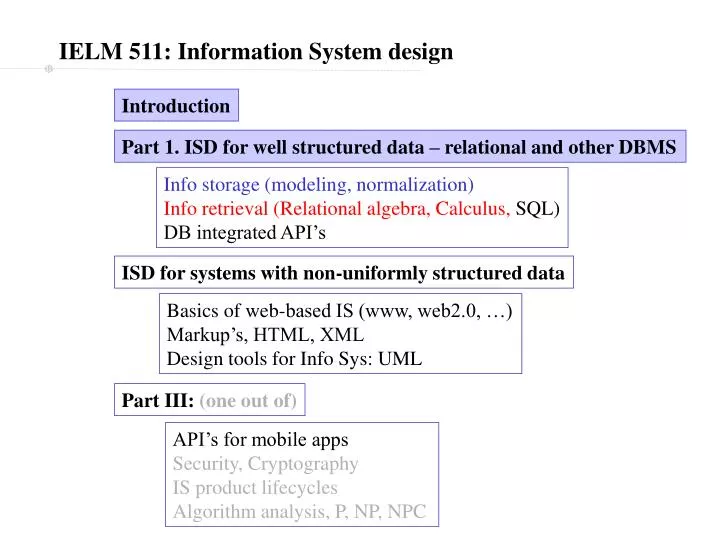
1. IELM 511: Information System design Introduction Part 1. ISD for well structured data – relational and other DBMS Info storage (modeling, normalization) Info retrieval (Relational algebra, Calculus, SQL) DB integrated API’s ISD for systems with non-uniformly structured data Basics of web-based IS (www, web2.0, …) Markup’s, HTML, XML Design tools for Info Sys: UML Part III: (one out of) API’s for mobile apps Security, Cryptography IS product lifecycles Algorithm analysis, P, NP, NPC

2. Agenda Relational Algebra Relational Calculus Structured Query Language (SQL) DB API’s

3. Recall our Bank DB design BRANCH( b-name, city, assets) CUSTOMER( cssn, c-name, street, city, banker, banker-type) LOAN( l-no, amount, br-name) PAYMENT(l-no, pay-no, date, amount) EMPLOYEE( e-ssn, e-name, tel, start-date, mgr-ssn) ACCOUNT( ac-no, balance) SACCOUNT( ac-no, int-rate) CACCOUNT( ac-no, od-amt) BORROWS(cust-ssn, loan-num) DEPOSIT(c-ssn, ac-num, access-date) DEPENDENT(emp-ssn, dep-name)

4. Background: Algebra What is an algebra ? Study of systems of mathematical objects and operations defined on the objects Examples of algebras: Integers, with operations: +, -, ×, /, % … Real numbers, with operations: +, -, ×, /, … Vectors, with operations: +, -, , ×, … Booleans, with operations: , , , …

5. Relational Algebra Relational Algebra: objects: instances of relational schemas (namely, tables) operations: s, P, ×, set-theoretic operations: , , -, ÷ Key concepts: Operator arguments: Arguments of operators are instances of schemas (table) Operation closure: The outcome of the operator is an instance of schema Expressions: A sequence of operations can be written as an expression Operator precedence: The sequence of application of operations in an expression is fixed. Compare these concepts to those in other algebras

6. Relational Algebra: select, s Notation: in remainder, we will refer to an instance of a schema as a table s : unary operator, input: one table; output: table LOAN s[amount > 1200](LOAN)

7. Relational Algebra: select, s q conditions of s operator: - Denote the criterion for selection of a given tuple - Must be evaluated one tuple at a time - Must evaluate to ‘true’ or ‘false’ - Output = set of tuples for which q-conditions are ‘true’ LOAN s[(amount > 1200)  (branch_name = ‘Pennyridge’)] (LOAN)

8. Relational Algebra: project, P P : unary operator, input: one table; output: table P[list of attributes] (TABLE) P[loan_number, amount] (LOAN) LOAN

9. Relational Algebra: project, P Project returns a set of tuples; the number of rows may be smaller that input Example: Find the names of all branches that have given loans P[branch_name] (LOAN) LOAN

10. Relational Algebra: combining operations Example: Find the names of all branches that have given loans larger than 1200 P[branch_name] ( s[(amount > 1200) ] (LOAN)) LOAN

11. Relational Algebra: combining operations Note: expressions impose a sequence in which operations are perfromed Example: Find the names of all branches that have given loans larger than 1200 X = ( s[(amount > 1200) ] (LOAN)) Y = P[branch_name] (X) Y X LOAN

12. Relational Algebra: join, × Join is useful when the information required is in two (or more) tables. Tables are sets of tuples, and the join of two tables produces a cartesian product of the two sets Background (set theory): cartesian product, A × B = { (x, y) | x  A, y  B} Example: A = { 1, 2, 3 }, B = { a, s} A × B = { (1, a), (1, s), (2, a), (2, s), (3, a), (3, s) }

13. Relational Algebra: join, × BORROWS LOAN 5 columns Cartesian product, BORROWS × LOAN 48 rows

14. Relational Algebra: join, × Usually, a cartesian product produces several tuples with un-related information. q-join specifies a q-condition (same as a selection criterion) to restrict the output of a join to meaningful tuples only. Example: Find the loan no, amount and branch name for all customers. BORROWS ×[loan_no = loan_number] LOAN 5 columns 8 rows [Why ?]

15. Relational Algebra: dot-notation in join, × Two tables being joined may have the same attribute name (possibly denoting two different things). To distinguish the columns in the q-join, the names of attributes use dot-notation The following are all equivalent: C = BORROWS ×[loan_no = loan_number] LOAN C = BORROWS ×[BORROWS.loan_no = LOAN.loan_number] LOAN A = BORROWS B = LOAN C = A ×[A.loan_no = B.loan_number] B

16. Relational Algebra: set theoretic operations,  Since a table is a set of tuples, it is possible to make a union of two tables. BUT: we require closure (union of two tables should be a table).  Union is defined for two tables with identical schemas. Example: Find the names of customers who have either a deposit, or a loan with the bank A = P[customer] (BORROWS) P[c_ssn] (DEPOSIT) RESULT = P[name] (A ×[A.customer= CUSTOMER.ssn] CUSTOMER )

17. Relational Algebra: set theoretic operations,  Other set theoretic operations can be applied with same rules. Example: Find the names of customers who have both, a deposit and a loan with the bank A = P[customer] (BORROWS) P[c_ssn] (DEPOSIT) RESULT = P[name] (A ×[A.customer= CUSTOMER.ssn] CUSTOMER ) RESULT  =

18. Relational Algebra: set theoretic operations, - Other set theoretic operations (same rules). Example: Find the names of customers who have a loan but no deposits. A = P[customer] (BORROWS) -P[c_ssn] (DEPOSIT) RESULT = P[name] (A ×[A.customer= CUSTOMER.ssn] CUSTOMER ) RESULT - =

19. Relational Algebra: set theoretic operations, ÷ Set division extends the meaning of integer division, in the sense that it ‘cancels away’ common multiples. It is useful in answering ‘for all’ queries. Example: Do all the loan officers have the same manager ? A solution: Find the ssn of the person who manages all the loan officers. A = P[banker] (s[b_type=LO] (CUSTOMER) ) B = P[mgr_ssn, e_ssn] (EMPLOYEE) RESULT = B ÷ A A B RESULT ÷ Note: for this example, we have to specify that the common divisor in B is e_ssn.

20. Relational Algebra: set theoretic operations, ÷ Generic definition of ÷ Attribute restrictions: A ÷ B is defined only for A( R, C) and B( C), where R, C are sets of attributes. Output: The output contains each ti[R] such that  tuples tj[C]  B,  a tuple, t  A in which t[C] = tj[C] and t[R] = ti[R]. common attribute set, C OUTPUT attribute set, R ÷ t1 … tn

21. Relational Algebra: concluding remarks RA provides a formal language to get information from the database RA can potentially answer any query, as long as the query pertains to exactly one row of some table derivable using expressions. Limitations of RA: aggregation and summary information Examples: find the average amount of assets in the branches find the total assets of the bank, … RA is procedural, namely, an expression of RA specifies a step by step procedure for computing the result.

22. Relational Calculus (RC) Background: what is a calculus ? RC is based on a formal system in logic, first order predicate calculus (fopc) A formal system has: a set of symbols; rules about how the symbols can be arranged in well formed formulae (wff) a (logical) mechanism to derive if a wff is true/false. additionally, fopc allows wff with ‘variables’ and quantifiers (, ). A query in RC takes the form: {t | P(t) } Meaning: the set of all tuples, t, for which some Proposition, P(t) is true. P is also called a predicate.

23. Relational Calculus (RC) examples 1. Report the loans that exceed $1200: { t | t  LOAN  t[amount] > 1200} 2. Find the names of customers who took a loan from the Pennyridge branch. { t[name] |  s  BORROWS  s[customer] = t[ssn]  u  LOAN  u[loan_number] = s[loan_no]  u[branch_name] = ‘Pennyridge’}

24. Relational Calculus (RC) remarks RC is non-procedural – any way that the predicate P can be evaluated is valid. RC is the formal basis for Structured Query Language (SQL) SQL is the de facto standard language for all RDBMSs In terms of functionality (i.e. the power to get some information from any DB) RA and RC are equivalent). Namely, any query that can be written in RC has an equivalent RA formula, and vice versa. Advantage of RC (over RA): conceptually, it is better to allow the user to define the logic of the query, but leave the procedure for computing it to the program [why ?].

25. Bank tables.. BRANCH EMPLOYEE

26. CUSTOMER DEPOSIT BORROWS LOAN

27. References and Further Reading Silberschatz, Korth, Sudarshan, Database Systems Concepts, McGraw Hill Next: SQL and DB API’s