Pipelining V
Pipelining V. Systems I. Topics Branch prediction State machine design. Branch Prediction. Until now - we have assumed a “predict taken” strategy for conditional branches Compute new branch target and begin fetching from there If prediction is incorrect, flush pipeline and begin refetching

Pipelining V
E N D
Presentation Transcript
Pipelining V Systems I Topics • Branch prediction • State machine design
Branch Prediction Until now - we have assumed a “predict taken” strategy for conditional branches • Compute new branch target and begin fetching from there • If prediction is incorrect, flush pipeline and begin refetching However, there are other strategies • Predict not-taken • Combination (quasi-static) • Predict taken if branch backward (like a loop) • Predict not taken if branch forward
Fetch Logic Revisited • During Fetch Cycle • Select PC • Read bytes from instruction memory • Examine icode to determine instruction length • Increment PC • Timing • Steps 2 & 4 require significant amount of time
Standard Fetch Timing • Must Perform Everything in Sequence • Can’t compute incremented PC until know how much to increment it by need_regids, need_valC Select PC Mem. Read Increment 1 clock cycle
Fast Slow A Fast PC Increment Circuit incrPC High-order 29 bits Low-order 3 bits carry MUX 0 1 29-bit incre- menter 3-bit adder need_regids 0 High-order 29 bits need_ValC Low-order 3 bits PC
Modified Fetch Timing • 29-Bit Incrementer • Acts as soon as PC selected • Output not needed until final MUX • Works in parallel with memory read need_regids, need_valC 3-bit add Select PC Mem. Read MUX Incrementer Standard cycle 1 clock cycle
More Realistic Fetch Logic • Fetch Box • Integrated into instruction cache • Fetches entire cache block (16 or 32 bytes) • Selects current instruction from current block • Works ahead to fetch next block • As reaches end of current block • At branch target
Instruction Control • Grabs Instruction Bytes From Memory • Based on Current PC + Predicted Targets for Predicted Branches • Hardware dynamically guesses whether branches taken/not taken and (possibly) branch target • Translates Instructions Into Operations • Primitive steps required to perform instruction • Typical instruction requires 1–3 operations • Converts Register References Into Tags • Abstract identifier linking destination of one operation with sources of later operations
Prediction Register Operations OK? Updates Integer/ General FP FP Functional Load Store Branch Integer Add Mult /Div Units Operation Results Addr . Addr . Data Data Data Cache Execution Execution ExecutionUnit • Multiple functional units • Each can operate in independently • Operations performed as soon as operands available • Not necessarily in program order • Within limits of functional units • Control logic • Ensures behavior equivalent to sequential program execution
CPU Capabilities of Intel iCore7 • Multiple Instructions Can Execute in Parallel • 1 load • 1 store • 1 FP multiplication or division • 1 FP addition • > 1 integer operation • Some Instructions Take > 1 Cycle, but Can be Pipelined • Instruction Latency Cycles/Issue • Load / Store 3 1 • Integer Multiply 3 1 • Integer Divide 11—21 5—13 • Double/Single FP Multiply 41 • Double/Single FP Add 3 1 • Double/Single FP Divide 10—15 6—11
iCore Operation • Translates instructions dynamically into “Uops” • ~118 bits wide • Holds operation, two sources, and destination • Executes Uops with “Out of Order” engine • Uop executed when • Operands available • Functional unit available • Execution controlled by “Reservation Stations” • Keeps track of data dependencies between uops • Allocates resources
High-Perforamnce Branch Prediction • Critical to Performance • Typically 11–15 cycle penalty for misprediction • Branch Target Buffer • 512 entries • 4 bits of history • Adaptive algorithm • Can recognize repeated patterns, e.g., alternating taken–not taken • Handling BTB misses • Detect in ~cycle 6 • Predict taken for negative offset, not taken for positive • Loops vs. conditionals
Branching Structures Predict not taken works well for “top of the loop” branching structures Loop: cmpl %eax, %edx je Out 1nd loop instr . . last loop instr jmp Loop Out: fall out instr • But such loops have jumps at the bottom of the loop to return to the top of the loop – and incur the jump stall overhead Predict not taken doesn’t work well for “bottom of the loop” branching structures Loop: 1st loop instr 2nd loop instr . . last loop instr cmpl %eax, %edx jne Loop fall out instr
Branch Prediction Algorithms Static Branch Prediction • Prediction (taken/not-taken) either assumed or encoded into program Dynamic Branch Prediction • Uses forms of machine learning (in hardware) to predict branches • Track branch behavior • Past history of individual branches • Learn branch biases • Learn patterns and correlations between different branches • Can be very accurate (95% plus) as compared to less than 90% for static
Predict branch based on past history of branch Branch history table Indexed by PC (or fraction of it) Each entry stores last direction that indexed branch went (1 bit to encode taken/not-taken) Table is a cache of recent branches Buffer size of 4096 entries are common (track 4K different branches) Simple Dynamic Predictor PC IR IM BHT Prediction update
Problem with a single bit • Imagine a heavily taken branch • It will be taken, taken, taken, but eventually not taken • Its predictor state will be N (not taken) • When we reexecute this branch, most likely we are in a new loop iteration. The branch is likely taken. • So mispredict on the first branch in the loop. • Then predict correctly for the entire loop. • But the exit condition will also be a mispredict. • Can we get down to 1 mispredict per loop execution?
Replace simple table of 1 bit histories with table of 2 bit state bits State transition logic can be shared across all entries in table Read entry out Apply combinational logic Write updated state bits back into table Enhanced Dynamic Predictor PC IR IM BHT Prediction update
A ‘predict same as last’ strategy gets two mispredicts on each loop Predict NTTT…TTT Actual TTTT…TTN Can do much better by adding inertia to the predictor e.g., two-bit saturating counter Predict TTTT…TTT Use two bits to encode: Strongly taken (T2) Weakly taken (T1) Weakly not-taken (N1) Strongly not-taken (N2) for(j=0;j<30;j++) { … } T T T T N2 N1 T1 T2 N N N N Multi-bit predictors State diagram to representing states and transitions
T T T T N2 N1 T1 T2 N N N N Comb.Logic State Variables(Flip-flops) How do we build this in Hardware? This is a sequential logic circuit that can be formulated as a state machine • 4 states (N2, N1, T1, T2) • Transitions between the states based on action “b” General form of state machine: inputs outputs
State Machine for Branch Predictor 4 states - can encode in two state bits <S1, S0> • N2 = 00, N1 = 01, T1 = 10, T2 = 11 • Thus we only need 2 storage bits (flip-flops in last slide) Input: b = 1 if last branch was taken, 0 if not taken Output: p = 1 if predict taken, 0 if predict not taken Now - we just need combinational logic equations for: • p, S1new, S0new, based on b, S1, S0
Combinational logic for state machine p =1 if state is T2 or T1 thus p = S1 (according to encodings) The state variables S1, S0 are governed by the truth table that implements the state diagram • S1new = S1*S0 + S1*b + S0*b • S0new = S1*S0’ + S0’*S1’*b + S0*S1*b
Misprediction rates (H&Pv4) • Predict taken • 34% for SPEC92 • Static profiling • 15% SD 5% for SPEC92INT • 9% SD 4% for SPEC92FP • Two bit predictor • 11% for SPEC89INT • 1024 10-bit global + 1K local entries (Alpha 21264) • 14% for SPEC95INT (29KB of state)
YMSBP Yet more sophisticated branch predictors Predictors that recognize patterns • eg. if last three instances of a given branches were NTN, then predict taken Predictors that correlate between multiple branches • eg. if the last three instances of any branch were NTN, then predict taken Predictors that correlate weight different past branches differently • e.g. if the branches 1, 4, and 8 ago were NTN, then predict taken Hybrid predictors that are composed of multiple different predictors • e.g. two different predictors run in parallel and a third predictor predicts which one to use More sophisticated learning algorithms
Branch target buffers Predictor tells us taken/not-taken • Actual target address still must be calculated Branch target buffer contains the predicted target address • Allows speculative fetch to occur earlier in pipeline • Requires more storage (PC, not just prediction state)
Summary Today • Branch mispredictions cost a lot in performance • CPU Designers willing to go to great lengths to improve prediction accuracy • Predictors are just state machines that can be designed using combinational logic and flip-flops