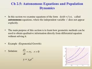
Ch 2.5: Autonomous Equations and Population Dynamics

1. Ch 2.5: Autonomous Equations and Population Dynamics • In this section we examine equations of the form dy/dt = f (y), called autonomous equations, where the independent variable t does not appear explicitly. • The main purpose of this section is to learn how geometric methods can be used to obtain qualitative information directly from differential equation without solving it. • Example (Exponential Growth): • Solution:

2. Logistic Growth • An exponential model y' = ry, with solution y = ert, predicts unlimited growth, with rate r > 0 independent of population. • Assuming instead that growth rate depends on population size, replace r by a function h(y) to obtain dy/dt = h(y)y. • We want to choose growth rate h(y) so that • h(y)  r when y is small, • h(y) decreases as y grows larger, and • h(y) < 0 when y is sufficiently large, (i.e. Population decreases) The simplest such function is h(y) = r – ay, where a > 0. • Our differential equation then becomes • This equation is known as the Verhulst, or logistic, equation.

3. Logistic Equation • The logistic equation from the previous slide is • This equation is often rewritten in the equivalent form where K = r/a. The constant r is called the intrinsic growthrate, and as we will see, K represents the carrying capacity of the population. • A direction field for the logistic equation with r = 1 and K = 10 is given here.

4. Logistic Equation: Equilibrium Solutions • Our logistic equation is • Two equilibrium solutions are clearly present: • In direction field below, with r = 1, K = 10, note behavior of solutions near equilibrium solutions: y = 0 is unstable, y = 10 is asymptotically stable.

5. Autonomous Equations: Equilibrium Solutions • Equilibrium solutions of a general first order autonomous equation y' = f (y) can be found by locating roots of f (y) = 0. • These roots of f (y) are called critical points. • For example, the critical points of the logistic equation are y = 0 and y = K. • Thus critical points are constant functions (equilibrium solutions) in this setting. (Question) How do we find the vertex of f(y) and its graph?

6. Logistic Equation: Qualitative Analysis and Curve Sketching (1 of 7) • To better understand the nature of solutions to autonomous equations, we start by graphing f (y) vs y. • In the case of logistic growth, that means graphing the following function and analyzing its graph using calculus.

7. Logistic Equation: Critical Points (2 of 7) • The intercepts of f occur at y = 0 and y = K, corresponding to the critical points of logistic equation. • The vertex of the parabola is (K/2, rK/4), as shown below.

8. Logistic Solution: Increasing, Decreasing (3 of 7) • Note dy/dt > 0 for 0 < y < K, so y is an increasing function of tthere (indicate with right arrows along y-axis on 0 < y < K). • Similarly, y is a decreasing function of t for y > K (indicate with left arrows along y-axis on y > K). • In this context the y-axis is often called the phase line.

9. Logistic Solution: Steepness, Flatness (4 of 7) • Note dy/dt 0 when y  0 or y  K, so y is relatively flat there, and y gets steep as y moves away from 0 or K.

10. Logistic Solution: Concavity (5 of 7) • Next, to examine concavity of y(t), we find y'': • Thus the graph of y is concave up when f and f' have same sign, which occurs when 0 < y < K/2 and y > K. • The graph of y is concave down when f and f' have opposite signs, which occurs when K/2 < y < K. • Inflection point occurs at intersection of y and line y = K/2.

11. (Example 1) Consider the logistic equation: K = 10 (1) Find equilibrium solutions (2) Find a general solution of the ODE • Hint: Use partial fractions

12. Solving the Logistic Equation • Provided y 0 and y K, we can rewrite the logistic ODE: • Expanding the left side using partial fractions, • Thus the logistic equation can be rewritten as • Integrating the above result, we obtain

13. Solving the Logistic Equation (2 of 3) • We have: • If 0 < y0 < K, then 0 < y < K and hence • Rewriting, using properties of logs:

14. Solution of the Logistic Equation (3 of 3) • We have: for 0 < y0 < K. • It can be shown that solution is also valid for y0 > K. Also, this solution contains equilibrium solutions y = 0 and y = K. • Hence solution to logistic equation is

15. Logistic Solution: Asymptotic Behavior • The solution to logistic ODE is • We use limits to confirm asymptotic behavior of solution: • Thus we can conclude that the equilibrium solution y(t) = K is asymptotically stable, while equilibrium solution y(t) = 0 is unstable. • The only way to guarantee solution remains near zero is to make y0 = 0.

16. Logistic Solution: Curve Sketching (6 of 7) • Combining the information on the previous slides, we have: • Graph of yincreasing when 0 < y < K. • Graph of ydecreasing when y > K. • Slope of y approximately zero when y  0 or y  K. • Graph of y concave up when 0 < y < K/2 and y > K. • Graph of y concave down when K/2 < y < K. • Inflection point when y = K/2. • Using this information, we can sketch solution curves y for different initial conditions.

17. Logistic Solution: Discussion (7 of 7) • Using only the information present in the differential equation and without solving it, we obtained qualitative information about the solution y. • For example, we know where the graph of y is the steepest, and hence where y changes most rapidly. Also, y tends asymptotically to the line y = K, for large t. • The value of K is known as the carrying capacity, or saturation level, for the species. • Note how solution behavior differs from that of exponential equation, and thus the decisive effect of nonlinear term in logistic equation.

18. Example 2: Pacific Halibut (1 of 2) • Let the halibut population in the pacific ocean satisfy the logistic equation with r = 0.71/year, K = 80.5 x 106 kg and y0 = 0.25K. Let y be biomass (in kg) of halibut population at time t. (a) Set up an ODE and solve the equation (b) Find the population 2 years later : (c) Find the time  such that y() = 0.75K.

19. Ex 2: Pacific Halibut (1 of 2) • Let y be biomass (in kg) of halibut population at time t, with r = 0.71/year and K = 80.5 x 106 kg. If y0 = 0.25K, find (a) biomass 2 years later (b) the time  such that y() = 0.75K. (a) For convenience, scale equation: Then and hence

20. Example 1: Pacific Halibut, Part (b) (2 of 2) (b) Find time  for which y() = 0.75K.

21. Critical Threshold Equation (1 of 2) • Consider the following modification of the logistic ODE: • The graph of the right hand side f (y) is given below.

22. Critical Threshold Equation: Qualitative Analysis and Solution (2 of 2) • Performing an analysis similar to that of the logistic case, we obtain a graph of solution curves shown below. • T is a threshold value for y0, in that population dies off or grows unbounded, depending on which side of T the initial value y0is. • See also laminar flow discussion in text. • It can be shown that the solution to the threshold equation is

23. Logistic Growth with a Threshold (1 of 2) • In order to avoid unbounded growth for y > T as in previous setting, consider the following modification of the logistic equation: • The graph of the right hand side f (y) is given below.

24. Logistic Growth with a Threshold (2 of 2) • Performing an analysis similar to that of the logistic case, we obtain a graph of solution curves shown below right. • T is threshold value for y0, in that population dies off or grows towards K, depending on which side of T y0is. • K is the carrying capacity level. • Note: y = 0 and y = K are stable equilibrium solutions, and y = T is an unstable equilibrium solution.