Download
1 / 26
270 likes | 771 Views
1st level analysis: basis functions, parametric modulation and correlated regressors . 1 st of February 2012 Sylvia Kreutzer Max-Philipp Stenner. First Level Analysis. Data analysis with SPM Pre-processing of the data (Alignment, smoothing etc .) First Level Analysis

E N D
1st level analysis: basis functions, parametric modulation and correlated regressors. 1st of February 2012 Sylvia Kreutzer Max-Philipp Stenner Methods for Dummies 2011/2012
First Level Analysis • Data analysis with SPM • Pre-processing of the data (Alignment, smoothing etc.) • First Level Analysis • Basis Functions (Sylvia) • Experimental design and correlated regressors(Max) • Random Field theory (next talk) • Second Level Analysis Methods for Dummies 2011/2012
Image time-series Statistical Parametric Map Design matrix Spatial filter Realignment Smoothing General Linear Model StatisticalInference RFT Normalisation p <0.05 Anatomicalreference Parameter estimates
Basis Functions • Temporal basis functions are used to model a more complex function • Function of interest in fMRI • Percent signal change over time • How to approximate the signal? • We have to find the combination of functions that give the best representation of the measured BOLD response • Default in SPM: Canonical hemodynamic response function (HDRF) Methods for Dummies 2011/2012
Basis Functions • Many different possible functions can be used f(t) h1(t) h2(t) h3(t) Fourier analysis The complex wave at the top can be decomposed into the sum of the three simpler waves shown below. f(t)=h1(t)+h2(t)+h3(t) Finite Impulse Response (FIR) Methods for Dummies 2011/2012
Peak Brief Stimulus Undershoot Initial Undershoot Hemodynamic Response Function (HRF) Since we know the shape of the hemodynamic response, we should use this knowledge and find a similar function to model the percentage signal change over time. This is our best prediction of the signal. Hemodynamic response function Methods for Dummies 2011/2012
Hemodynamic Response Function(HRF) Two gamma functions added together form a good representation of the haemodynamic response, although they lack the initial undershoot! Gamma functions Two Gamma functions added Methods for Dummies 2011/2012
Limits of HRF • General shape of the BOLD impulse response similar across early sensory regions, such as V1 and S1. • Variability across higher cortical regions. • Considerable variability across people. • These types of variability can be accommodated by expanding the HRF...
Canonical HRF Temporal derivative Dispersion derivative Informed Basis Set • Canonical HRF (2 gamma functions) plus two expansions in: • Time: The temporal derivative can model (small) differences in the latency of the peak response • Width: The dispersion derivative can model (small) differences in the duration of the peak response. Methods for Dummies 2011/2012
Left Right Mean Design Matrix 3 regressors used to model each condition The three basis functions are: 1. Canonical HRF 2. Derivatives with respect to time 3. Derivatives with respect to dispersion Methods for Dummies 2011/2012
Ex: Auditory words every 20s Gamma functions ƒi() of peristimulus time SPM{F} Sampled every TR = 1.7s Design matrix, X [x(t)ƒ1() | x(t)ƒ2() |...] … 0 time {secs} 30 General (convoluted) Linear Model REVIEW DESIGN
Comparison of the fitted response Haemodynamic response in a single voxel. Left: Estimation using the simple model Right: More flexible model with basis functions Methods for Dummies 2011/2012
Summary SPM uses basis functions to model the hemodynamic response using a single basis function or a set of functions. The most common choice is the `Canonical HRF' (Default in SPM) By adding the time and dispersion derivatives one can account for variability in the signal change over voxels Methods for Dummies 2011/2012
Sources • www.mrc-cbu.cam.ac.uk/Imaging/Common/rikSPM-GLM.ppt • http://www.fil.ion.ucl.ac.uk/spm/doc/manual.pdf • And thanks to Guillaume! Methods for Dummies 2011/2012
Part II: Correlated regressorsparametric/non-parametric design Methods for Dummies 2011/2012
Multicollinearity yi= ß0 + ß1xi1+ ß2xi2+… + ßNxiN+ e Coefficients reflect an estimated change in y with every unit change in xi while controlling for all other regressors Methods for Dummies 2011/2012
Multicollinearity { yi = ß0+ ß1xi1 + ß2xi2+… + ßNxiN + e xi1 = l0 + lxi2 + v low variance of v high variance of v Xi1 (e.g. age) Xi1 x x x x x x x x x x x x x x x x x x x x x x Xi2 Xi2 (e.g. chronic disease duration) Methods for Dummies 2011/2012
y e x2 x1 Multicollinearity and estimability • OLS minimizes e by • Xe = 0 • with • e = Y – (Xbestim)-1 • which gives • bestim= (XTX)-1XTY (SPM course Oct. 2010, Guillaume Flandin) cf covariance matrix • high multicollinearity • (i.e. variance of v small) • inaccuracy of individual bestim, high standard error • perfect multicollinearity • (i.e. variance of v = 0) • det(X) = 0 • (XTX) not invertible • bestimnot unique Methods for Dummies 2011/2012
Multicollinearity • (t- and [unidimensional] F-) testing of a single regressor (e.g. R1) =̂ testing for the component that is not explained by (is orthogonal to) the other/the reduced model (e.g. R2) • multicollinearity is contrast specific • “conflating” correlated regressors by means of (multidimensional) F-contrasts permits assessing common contribution to variance • (Xibestim= projection of Yi onto X space) R1’ Xibestim R1 R2 Methods for Dummies 2011/2012
Multicollinearity (relatively) little spread after projection onto x-axis, y-axis or f(x) = x reflecting reduced efficiency for detecting dependencies of the observed data on the respective (combination of) regressors regressor 2 x hrf regressor 1 x hrf (MRC CBU Cambridge, http://imaging.mrc-cbu.cam.ac.uk/imaging/DesignEfficiency) Methods for Dummies 2011/2012
Orthogonality matrix reflects the cosine of the angles between respective pairs of columns (SPM course Oct. 2010, Guillaume Flandin) Methods for Dummies 2011/2012
Orthogonalizing leaves the parameter estimate of R1 unchanged but alters the estimate of the R2 parameter assumes unambiguous causality between the orthogonalized predictor and the dependent variable by attributing the common variance to this one predictor only hence rarely justified Xbestim R1orth R1 R2 R2new Methods for Dummies 2011/2012
Dealing with multicollinearity • Avoid. • (avoid dummy variables; when • sequential scheme of predictors • (stimulus – response) is inevitable: • inject jittered delay (see B) or use a • probabilistic R1-R2 sequence (see C)) • Obtain more data to decrease standard error of parameter estimates • Use F-contrasts to assess common contribution to data variance • Orthogonalizing might lead to self-fulfilling prophecies (MRC CBU Cambridge, http://imaging.mrc-cbu.cam.ac.uk/imaging/DesignEfficiency) Methods for Dummies 2011/2012
Parametric vs. factorial design Widely-used example (Statistical Parametric Mapping, Friston et al. 2007) Four button press forces factorial parametric Methods for Dummies 2011/2012
Parametric vs. factorial design Which– when? Limited prior knowledge, flexibility in contrasting beneficial (“screening”): Large number of levels/continuous range: factorial parametric Methods for Dummies 2011/2012
Happy mapping! Methods for Dummies 2011/2012