Finite Elements: Basis functions

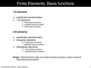
1. Finite Elements: Basis functions 1-D elements coordinate transformation 1-D elements linear basis functions quadratic basis functions cubic basis functions 2-D elements coordinate transformation triangular elements linear basis functions quadratic basis functions rectangular elements linear basis functions quadratic basis functions Scope: Understand the origin and shape of basis functions used in classical finite element techniques.

2. 1-D elements: coordinate transformation We wish to approximate a function u(x) defined in an interval [a,b] by some set of basis functions where i is the number of grid points (the edges of our elements) defined at locations xi. As the basis functions look the same in all elements (apart from some constant) we make life easier by moving to a local coordinate system so that the element is defined for x=[0,1].

3. 1-D elements – linear basis functions There is not much choice for the shape of a (straight) 1-D element! Notably the length can vary across the domain. We require that our function u(x) be approximated locally by the linear function Our node points are defined at x1,2=0,1 and we require that

4. 1-D elements – linear basis functions As we have expressed the coefficients ci as a function of the function values at node points x1,2 we can now express the approximate function using the node values .. and N1,2(x) are the linear basis functions for 1-D elements.

5. 1-D quadratic elements Now we require that our function u(x) be approximated locally by the quadratic function Our node points are defined at x1,2,3=0,1/2,1 and we require that

6. 1-D quadratic basis functions ... again we can now express our approximated function as a sum over our basis functions weighted by the values at three node points ... note that now we re using three grid points per element ... Can we approximate a constant function?

7. 1-D cubic basis functions ... using similar arguments the cubic basis functions can be derived as ... note that here we need derivative information at the boundaries ... How can we approximate a constant function?

8. 2-D elements: coordinate transformation y P3 P2 P1 x Let us now discuss the geometry and basis functions of 2-D elements, again we want to consider the problems in a local coordinate system, first we look at triangles h P3 x P2 P1 after before

9. 2-D elements: coordinate transformation h P1 (0,0) P3 P2 (1,0) P3 (0,1) P2 x P1 Any triangle with corners Pi(xi,yi), i=1,2,3 can be transformed into a rectangular, equilateral triangle with using counterclockwise numbering. Note that if h=0, then these equations are equivalent to the 1-D tranformations. We seek to approximate a function by the linear form we proceed in the same way as in the 1-D case

10. 2-D elements: coefficients h P1 (0,0) P3 P2 (1,0) P3 (0,1) P2 x P1 ... and we obtain ... and we obtain the coefficients as a function of the values at the grid nodes by matrix inversion containing the 1-D case

11. triangles: linear basis functions h P1 (0,0) P3 P2 (1,0) P3 (0,1) P2 x P1 from matrix A we can calculate the linear basis functions for triangles

12. triangles: quadratic elements h P1 (0,0) P2 (1,0) P3 P3 (0,1) + P4 (1/2,0) P5 (1/2,1/2) P5 + P6 P6 (0,1/2) + P2 + + + x P1 P4 Any function defined on a triangle can be approximated by the quadratic function and in the transformed system we obtain as in the 1-D case we need additional points on the element.

13. triangles: quadratic elements h P1 (0,0) P2 (1,0) P3 P3 (0,1) + P4 (1/2,0) P5 (1/2,1/2) P5 + P6 P6 (0,1/2) + P2 + + + x P1 P4 To determine the coefficients we calculate the function u at each grid point to obtain ... and by matrix inversion we can calculate the coefficients as a function of the values at Pi

14. triangles: basis functions h P1 (0,0) P2 (1,0) P3 P3 (0,1) + P4 (1/2,0) P5 (1/2,1/2) P5 + P6 P6 (0,1/2) + P2 + + + x P1 P4 ... to obtain the basis functions ... and they look like ...

15. triangles: quadratic basis functions h P1 (0,0) P2 (1,0) P3 P3 (0,1) + P4 (1/2,0) P5 (1/2,1/2) P5 + P6 P6 (0,1/2) + P2 + + + x P1 P4 The first three quadratic basis functions ...

16. triangles: quadratic basis functions h P1 (0,0) P2 (1,0) P3 P3 (0,1) + P4 (1/2,0) P5 (1/2,1/2) P5 + P6 P6 (0,1/2) + P2 + + + x P1 P4 .. and the rest ...

17. rectangles: transformation Let us consider rectangular elements, and transform them into a local coordinate system h y P3 P4 P3 P4 P2 P1 x x P2 P1 after before

18. rectangles: linear elements With the linear Ansatz we obtain matrix A as and the basis functions

19. rectangles: quadratic elements h P7 P3 P4 + + P6 + P8 + x P2 P1 P5 With the quadratic Ansatz we obtain an 8x8 matrix A ... and a basis function looks e.g. like N1 N2

20. 1-D and 2-D elements: summary The basis functions for finite element problems can be obtained by: • Transforming the system in to a local (to the element) system • Making a linear (quadratic, cubic) Ansatz for a function defined across the element. • Using the interpolation condition (which states that the particular basis functions should be one at the corresponding grid node) to obtain the coefficients as a function of the function values at the grid nodes. • Using these coefficients to derive the n basis functions for the n node points (or conditions).