Download
1 / 71
870 likes | 2.03k Views
Principles of Linear Pipelining. Principles of Linear Pipelining. In pipelining, we divide a task into set of subtasks. The precedence relation of a set of subtasks {T 1 , T 2 ,…, T k } for a given task T implies that the same task T j cannot start until some earlier task T i finishes.

E N D
Principles of Linear Pipelining • In pipelining, we divide a task into set of subtasks. • The precedence relation of a set of subtasks {T1, T2,…, Tk} for a given task T implies that the same task Tj cannot start until some earlier task Ti finishes. • The interdependencies of all subtasks form the precedence graph.
Principles of Linear Pipelining • With a linear precedence relation, task Tj cannot start until earlier subtasks { Ti} for all (i < j) finish. • A linear pipeline can process subtasks with a linear precedence graph.
Principles of Linear Pipelining • A pipeline can process successive subtasks if • Subtasks have linear precedence order • Each subtasks take nearly same time to complete
Basic Linear Pipeline • L: latches, interface between different stages of pipeline • S1, S2, etc. : pipeline stages
Basic Linear Pipeline • It consists of cascade of processing stages. • Stages:Pure combinational circuits performing arithmetic or logic operations over the data flowing through the pipe. • Stages are separated by high speed interface latches. • Latches : Fast Registers holding intermediate results between stages • Information Flow are under the control of common clock applied to all latches
Basic Linear Pipeline • L: latches, interface between different stages of pipeline • S1, S2, etc. : pipeline stages
Basic Linear Pipeline • The flow of data in a linear pipeline having four stages for the evaluation of a function on five inputs is as shown below:
Basic Linear Pipeline • The vertical axis represents four stages • The horizontal axis represents time in units of clock period of the pipeline.
Clock Period (τ) for the pipeline • Let τi be the time delay of the circuitry Si and t1 be time delay of latch. • Then the clock period of a linear pipeline is defined by • The reciprocal of clock period is called clock frequency (f = 1/τ) of a pipeline processor.
Performance of a linear pipeline • Consider a linear pipeline with k stages. • Let T be the clock period and the pipeline is initially empty. • Starting at any time, let us feed n inputs and wait till the results come out of the pipeline. • First input takes k periods and the remaining (n-1) inputs come one after the another in successive clock periods. • Thus the computation time for the pipeline Tp is Tp = kT+(n-1)T = [k+(n-1)]T
Performance of a linear pipeline • For example if the linear pipeline have four stages with five inputs. • Tp = [k+(n-1)]T = [4+4]T = 8T
Floating Point Adder Unit • This pipeline is linearly constructed with 4 functional stages. • The inputs to this pipeline are two normalized floating point numbers of the form A = a x 2p B = b x 2q where a and b are two fractions and p and q are their exponents. • For simplicity, base 2 is assumed
Floating Point Adder Unit • Our purpose is to compute the sum C = A + B = c x 2r = d x 2s where r = max(p,q) and 0.5 ≤ d < 1 • For example: A=0.9504 x 10³ B=0.8200 x 10² a = 0.9504 b= 0.8200 p=3 & q =2
Floating Point Adder Unit • Operations performed in the four pipeline stages are : • Compare p and q and choose the largest exponent, r = max(p,q)and compute t = |p – q| Example: r = max(p , q) = 3 t = |p-q| = |3-2|= 1
Floating Point Adder Unit • Shift right the fraction associated with the smaller exponent by t units to equalize the two exponents before fraction addition. • Example: Smaller exponent, b= 0.8200 Shift right b by 1 unit is 0.082
Floating Point Adder Unit • Perform fixed-point addition of two fractions to produce the intermediate sum fraction c, where 0 ≤ c < 1 • Example : a = 0.9504 b= 0.082 c = a + b = 0.9504 + 0.082 = 1.0324
Floating Point Adder Unit • Count the number of leading zeros (u) in fraction c and shift left c by u units to produce the normalized fraction sum d = c x 2u, with a leading bit 1. Update the large exponent s by subtracting s = r – u to produce the output exponent. • Example: c = 1.0324 , u = -1 right shift d = 0.10324 , s= r – u = 3-(-1) = 4 C = 0.10324 x 10⁴
Floating Point Adder Unit • The above 4 steps can all be implemented with combinational logic circuits and the 4 stages are: • Comparator / Subtractor • Shifter • Fixed Point Adder • Normalizer (leading zero counter and shifter)
4-STAGE FLOATING POINT ADDER p q A = a x 2 B = b x 2 a A b B Other Stages: Fraction Exponent fraction subtractor selector S1 Fraction with min(p,q) r = max(p,q) Right shifter t = |p - q| Fraction S2 adder c r Leading zero counter S3 c Left shifter r d Exponent adder S4 s d C= X + Y = d x 2s
Exponents Mantissas a b A B R R Difference=3-2=1 For example: X=0.9504*103 Y=0.8200*102 Compare exponents by subtraction Segment 1: Align mantissas 0.082 R R 3 Choose exponent Segment 2: Add mantissas S=0.9504+0.082=1.0324 Segment 3: R R 4 Adjust exponent Normalize result 0.10324 Segment 4: R R Example for floating-point adder
Performance Parameters • The various performance parameters of pipeline are : • Speed-up • Throughput • Efficiency
Speedup • Speedup is defined as Speedup = Time taken for a given computation by a non-pipelined functional unit Time taken for the same computation by a pipelined version • Assume a function of k stages of equal complexity which takes the same amount of time T. • Non-pipelined function will take kT time for one input. • Then Speedup = nkT/(k+n-1)T = nk/(k+n-1)
Speed-up • For e.g., if a pipeline has 4 stages and 5 inputs, its speedup factor is Speedup = ?
Efficiency • It is an indicator of how efficiently the resources of the pipeline are used. • If a stage is available during a clock period, then its availability becomes the unit of resource. • Efficiency can be defined as
Efficiency • No. of stage time units = nk • there are n inputs and each input uses k stages. • Total no. of stage-time units available = k[ k + (n-1)] • It is the product of no. of stages in the pipeline (k) and no. of clock periods taken for computation(k+(n-1)).
Throughput • It is the average number of results computed per unit time. • For n inputs, a k-staged pipeline takes [k+(n-1)]T time units • Then, Throughput = n / [k+n-1] T = nf / [k+n-1] where f is the clock frequency • Throughput = Efficiency x Frequency
Handler’s Classification • Based on the level of processing, the pipelined processors can be classified as: • Arithmetic Pipelining • Instruction Pipelining • Processor Pipelining
Arithmetic Pipelining • The arithmetic logic units of a computer can be segmented for pipelined operations in various data formats. • Example : Star 100
Instruction Pipelining • The execution of a stream of instructions can be pipelined by overlapping the execution of current instruction with the fetch, decode and operand fetch of the subsequent instructions • It is also called instruction look-ahead
Processor Pipelining • This refers to the processing of same data stream by a cascade of processors each of which processes a specific task • The data stream passes the first processor with results stored in a memory block which is also accessible by the second processor • The second processor then passes the refined results to the third and so on.
Li and Ramamurthy's Classification • According to pipeline configurations and control strategies, Li and Ramamurthy classify pipelines under three schemes • Unifunction v/s Multi-function Pipelines • Static v/s Dynamic Pipelines • Scalar v/s Vector Pipelines
Unifunctional Pipelines • A pipeline unit with fixed and dedicated function is called unifunctional. • Example: CRAY1 (Supercomputer - 1976) • It has 12 unifunctional pipelines described in four groups: • Address Functional Units: • Address Add Unit • Address Multiply Unit
Unifunctional Pipelines • Scalar Functional Units • Scalar Add Unit • Scalar Shift Unit • Scalar Logical Unit • Population/Leading Zero Count Unit • Vector Functional Units • Vector Add Unit • Vector Shift Unit • Vector Logical Unit
Unifunctional Pipelines • Floating Point Functional Units • Floating Point Add Unit • Floating Point Multiply Unit • Reciprocal Approximation Unit
Multifunctional A multifunction pipe may perform different functions either at different times or same time, by interconnecting different subset of stages in pipeline. Example 4X-TI-ASC (Supercomputer - 1973)
Static Pipeline • It may assume only one functional configuration at a time • Static pipelines are preferred when instructions of same type are to be executed continuously • A unifunction pipe must be static.
Dynamic pipeline • It permits several functional configurations to exist simultaneously • A dynamic pipeline must be multi-functional • The dynamic configuration requires more elaborate control and sequencing mechanisms than static pipelining
Scalar Pipeline • It processes a sequence of scalar operands under the control of a DO loop • Instructions in a small DO loop are often prefetched into the instruction buffer. • The required scalar operands are moved into a data cache to continuously supply the pipeline with operands • Example: IBM System/360 Model 91
Vector Pipelines • They are specially designed to handle vector instructions over vector operands. • Computers having vector instructions are called vector processors. • The design of a vector pipeline is expanded from that of a scalar pipeline. • The handling of vector operands in vector pipelines is under firmware and hardware control. • Example : Cray 1
3 stage non-linear pipeline Output A • It has 3 stages Sa, Sb and Sc and latches. • Multiplexers(cross circles) can take more than one input and pass one of the inputs to output • Output of stages has been tapped and used forfeedback and feed-forward. Output B Input Sa Sb Sc